What is path planning?

Path planning is taking some desired goal sequence of points and deriving some sort of solution for the robot that hits the points, or gets close to them. You have these position constraints, as well as velocity constraints and acceleration.

Joint Space vs Cartesian Space

In joint space, we have direct control over the joints, so anything in the workspace can be accessed. More specifically, if you have some set $\theta_1$ and some set $\theta_2$, any interpolation can be reached. A trajectory can be easily executed.

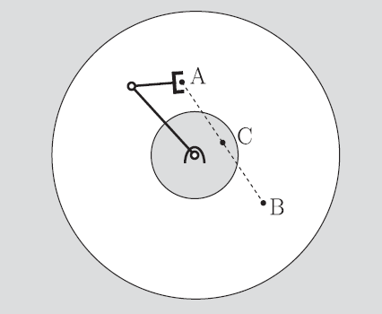
In cartesian space, you might actually run into situations where you can’t move in a straight line because there are some points that are outside of the work area.

You might get restrictions in both the joint and task space (joint space: limits. Task space: obstacles). These two spaces may have a very complicated relationship with each other.

Ways of solving

Direct solve: you can use a C-space method (don’t worry too much about this) but this gets you an exact solution for the allowable trajectories. The unfortunate realty is that this is inefficient and needs to be recomputed every time an object moves

You can also sample and check: if you have some joint configuration, you can run forward kinematics to see where you are, and if you’re avoiding the obstacle alright. You can continue in a stochastic way to generate a valid trajectory. This, of course, suffers from the curse of dimensionality.

Singularities

There are three types of singularities that a robot may encounter. First, it might encounter a point that it just can’t reach.

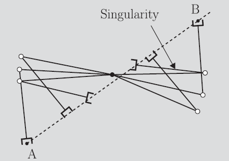
Second, if considering dynamics, it may encounter a stretch of the trajectory where maintaining some constant velocity may require an infinite joint velocity (see example below). More on this later.

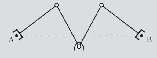
Third, all points may be reachable, but some of the points may require drastically different joint space solutions, which may require a flip in configuration.

More on this later, when we discuss the Jacobian.

Linear interpolation

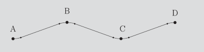
Let’s say that you have a set of points that you can move the robot through. How do you actually generate this path?

One idea is to just connect the dots with lines. This is ok but you get velocity discontinuities between the points that can be quite jarring for the robot (requires infinite torque, essentially)

Polynomial interpolation

So instead of linear interpolation, we need to add two more constraints: velocity constraints. To solve this problem, we need a polynomial curve.

You make each intermediate path a polynomial and join them at the points. Because the velocities are zero, you can splice the polynomials together without noticing anything.

Of course, the accelerations are discontinuous, and if you wanted to add another set of constraints, you need a fifth degree polynomial.

Polynomial trajectory: Between two points

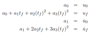
You may also try to hit these points using a higher-level polynomial like a cubic, which would avoid some of the hassle induced by blend curves. If you only had a set of start and end conditions, you can solve for these parameters as a system of linear equations (because the parameters themselves are non-polynomial)

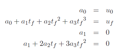
The first two constraints are start and end, and the last two constraints constrain the velocity to be zero at each of the points. Graphically, you can think of a robot arm starting from rest and slowing to a stop at the target point. There are no constraints on acceleration.

Polynomial trajectory: Planning with intermediates (via points)

Previously, we figured out how to go between two points. We can therefore go along a set of points by chaining them together. The only problem is that you would have to stop at each point, which doesn’t seem efficient. Can we have smooth motion?

As an initial idea, we could try just increasing the order of polynomials. This is ok but you could have some unwanted curves

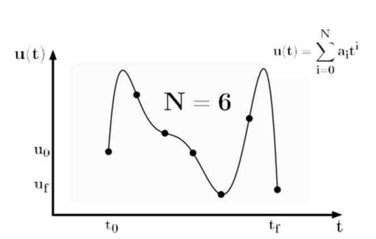
Or, you can just set a desired “idle” velocity for every waypoint and solve for this idle velocity.

Straight paths with Parabolic Blends (via points)

This is slightly more involved because you are basically making a piecewise function. You have a line of the format $a_0 + a_1 t$ that you’re splicing with a parabolic blend of type $\frac{1}{2}at^2$.

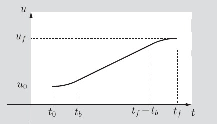
The math here is a bit involved, but you can imagine that you need to carefully match the derivatives. The benefit is that the acceleration will be zero for most of the path.

Further challenges

We talked about doing these polynomial paths independently for each joint, but if you want to trace out a specific curve in task space, you need multiple joints to be coordinated at once.

So if you really wanted to move in a very specific path in operational space, you may need to compute a ton of IK; there isn’t a really nice closed form solutoin to generate a trajectory in joint space.