This is supposed to be a very brief review of everything. I’ve only included the most important bits of information

Spatial Representation

Remember that vectors are technically agnostic to representation, but once you have to represent them, you need to be consistent with the format.

Rotation Matrix

Defined as three orthogonal vectors with determinant 1 that represents the new unit vectors after the rotation. It can represent all rotations.

General transformations

When we make a general transformation, we take everything into the desired frame (which means applying a rotation to the original vector)

We can represent this neatly using a Homogenous matrix

We typically denote this as $T$, and you can transform any point into any other frame using this approach.

You can invert this transformation by bringing everything into the inverted basis and then negating (this part is important)

Transformations as operators

If you read transformations from left to right, you can imagine doing the transformations to a base vector in a forward way, so $^A_BR$ would move a vector as if it were transforming from A to B.

Orientation Representation

We looked at the rotation matrix, let’s look at some other representations.

Euler angles

The euler angle is a composition of three transformations made along each transformed axis

So this would be a ZYX transformation. You can also read this as a fixed-angle transformation in XYZ (note how they are just read forward and backwards).

You can find the angles by computing the following (only for ZYX)

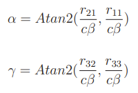
There are singularities, namely if $\cos(\beta) = 0$.

Axis angle representation

You represent the rotation as some axis and some angle around that axis. If you work it out, you’ll get

with a singularity when $\theta = 0$.

Quaternion

This is just the axis angle but it’s encoded in a more tricky way:

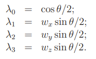
From a rotation matrix, you get this formula

And you can solve by looking at the sum of the diagonal elements. See main notes for more details.

Direct Kinematics

Links

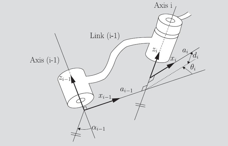
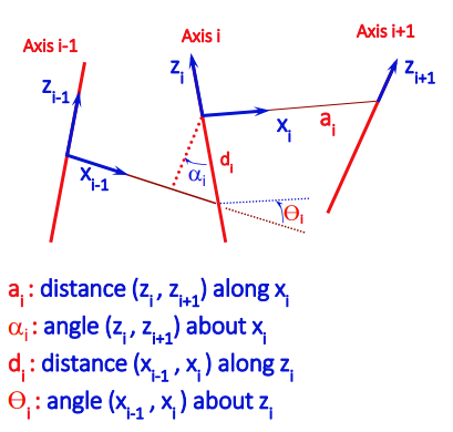
Links are always on the Z axis with the X axis pointing to the next link. Therefore, to travel from link to link, you align the Z axes and move the Z axes to align to the next axis (both rotations and translations along the x axis), and then you move / rotate along the new Z axis to propagate to the next joint. The two things along the x axis are $a, \alpha$, and the two things along the z axis is $d_i, \theta_i$. Note that this operation is on the current frame.

First link is typically placed to have the easiest interaction with $x_1, z_1$. The last link can be at the EEF, but it can also just be at the last joint.

Propagation of frames

To propagate frames, just do the x rotations and then the z rotations.

Inverse Kinematics

Geometric solutions

If the manipulator is simple enough, you may be able to draw some diagrams and find a neat relationship between $x, y$ and the joint parameters. This is only in special cases, as you often don’t get very lucky.

Algebraic solutions

This is when you express the whole transformation matrix and then you attempt to solve for the angles.

Trajectory generation

Polynomial generation

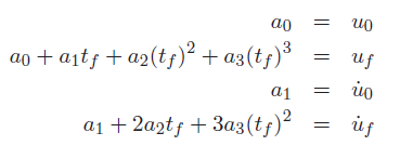
You just need to parameterize a cubic and constrain the starting and ending positions and velocities. This becomes a system of linear equations

Jacobian

The Jacobian tells us how the positions and angles would change with a perturbation of the joints

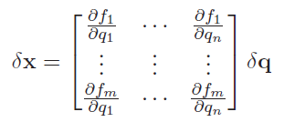
Note that each column is the perturbation WRT a single joint of all the x’s. You create two Jacobians: one for the positions, and one for the rotations

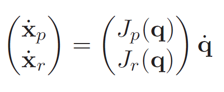
Linear and angular motion

For pure translation, velocity propagation is trivial:

For pure rotation, it is also trivial: just add the $\Omega$, which is the axis of rotation.

For translation and rotation, the rotation adds a linear component based on a cross product $\Omega \times p$

So it becomes

and if you need it in one frame, it is

Explicit form jacobian

If you have access to the $p_{in}$ vectors, it is just

and the rotation is

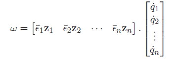
but in most cases, you have access to a transformation matrix. In that case, just manually take the derivative

Changing frames, moving end-effectors

To change frames, just apply rotation matrix (translation doesn’t matter for Jacobian, which is for changes)

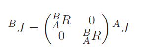
If you want to apply Jacobian at end-effector, usually it’s sufficient to add the appropiate amount to the $T$ matrix and take the derivative. In vector form, you just need (for the position jacobian)

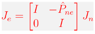
Singularity

Singularity is when you lose one degree of freedom. This may not be in an explicit axis, but it can be. You always express it in the end-effector frame (which is much easier).

Formally, this is when the determinant becomes zero. Remember that the determinant of a 3x3 matrix can be computed in different ways.

Forces

The torque is just the cross product of the radius and the force applied

To propagate forces, in static-land, you just need to equalize out the forces and torques. The torques are applied by the joints to oppose the torque applied on them. Positive is applying, negative is receiving.

Propagating forces

You start with the force applied at the end-effector. The robot’s starting force will be in opposition to this force (or, if it’s applying, this is the force that it’s applying). Then, you propagate backwards.

The jacobian relationship

If you look at the virtual work equation

You’ll derive the torque-force relationship

Forces in the nullspace of $J^T$ are supported but not exertable. Forces not in the nullspace exert torques on the joints

Dynamics

Dynamics is about how a system evolves through time. Inherently, dynamics is a differential equation. You get an equation of motion, like $F = ma$ that tells you the relationship between applied forces and resulting acceleration. When there are multiple joints involved, this relationship becomes quite complicated.

There are two main methods to formulate dynamics. There’s the direct euler method that computes all the matrices and things directly, or there is the Lagrange way that starts from energy. Both ways of understanding dynamics yields this equation of motion

This $\tau$ is applied force from the environment

Euler formulation

The idea here is to find momentum and take the time derivative to get force or a moment. The angular momentum of a rigid body is

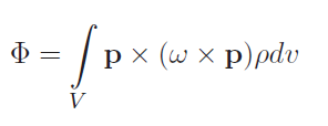
which means that the moment is defined as

The linear analog is just $F = (d/dt)mv$.

Moments of Inertia

As a side note, the Inertial tensor is defined as

which gets you an integration matrix that looks like this:

and you integrate each component against $\rho dxdydz$. Remember that a blank integration is just the difference of the end bounds of the integral.

If you want to find a different axis and it’s parallel, use he parallel axis theorem:

Or if you have a rotated frame, just frame the inertia around the rotation matrix

Energy formulation

We can start with the energy $L = K - V$. It turns out that this is the Lagrange, and there’s a famous Lagrange equation as follows:

This basically tells us the equation of motion if we can find these components. If you write out the formulation of kinetic energy

And this gets us the $M\ddot q + V(q, \dot q)$. If you write out the formulation for potential energy, you first get the gravity vector

and you get

so practically speaking, the negative signs actually cancel out and you get a fully positive pickup.

Writing out the mass matrix

So what exactly is the mass matrix? It seems like everything we need to know is in the mass matrix. Well, we can use an energy construction:

We have $\dot q$ and we can use the Jacobian to bring this expression to fruition

Naturally, each Jacobian doesn’t regard links after this link as contributing to the problem, which indicates that

To compute this, make sure that your frames for each $J$ are correct, although because energy is a scalar quantity, they don’t need to completely match. Tyipcally, $J_v$ is in frame 0, but $J_w$ is in the frame of $I_C$, which is typically referenced at the center of mass.

Centrifugal and Coriolis Forces

This is the $v(q, \dot q)$ component. Now, we already have enough to compute the matrix, but there is a special framework that explains what these components are. If we really do these derivatives out, we’ll get

and using Christoffel symbols, we can express this as

where

Things to watch out for

Gravity component is negative because we are dealing with a force that is being applied.

Make sure that you frames are correct.

Dot notation:

• $\dot M$ means that we take the time derivative of $M$. If you encounter some $f(q)$ inside, the derivative is $f’(q)\dot q$ (mind the difference)

• $dM/dq$ means that we take the derivative WRT $q$

• $dM/d\dot q$ means that we take the derivative WRT $\dot q$. Ignore cases of $q$.

Control

Control builds upon dynamics. If you have an equation of motion, you can run time forward and see what happens. This is when you set the applied torque equal to zero. But what happens if you set the applied torque equal to some function? Well, you get a new equation of motion. In some cases, if you set the functions carefully, you get some very neat properties.

In all of our analysis, we use the Lagrange energy formulation and the Lagrange equation. We don’t need to solve any PDEs because we assume one standard form of solution.

Spring-damper systems

If you had a conservative system and a spring that pulls you towards some destination, you have

which gets you this equation of motion

which gives the path

where $\omega = \sqrt{k/m}$. Now, with dissipative systems, we just add the dissipative force.

and if we have viscous friction, we get the form

Now, we have $\xi_n = b/(2\sqrt{km})$. This tells us the damping ratio (low → overdamped, high → overdamped, 1 = perfect). The resonance frequency is still $\omega = \sqrt{k/m}$.

We care about these systems because they are exactly how we might want to control our robot!

Asymptotic stability

A system is stable if it doesn’t get out of control. A system is marginally stable if it doesn’t get out of control but it also doesn’t settle down. A good example is a spring system with no friction. An asymptotic stable system always applies force that is at least perpendicular to the velocity

PD Control

PD control means setting $F = -k_p(x - x_d) - k_v \dot x$, which is equivalent to attaching a dampened spring to the system. This gets you the motion euation

and all the analysis on it are boilerplate. $\omega = \sqrt{k_p / m}$, and $\xi = k_v / (2\sqrt{k_p m})$.

We realize that the control is linear in the mass $m$, which means that it is common to create a unit mass controller and scale it up by a weight estimate: $f = m f’$.

Nonlinear control

In PD control, we assumed that the equation of motion is $m\ddot x = f$. But there could be other factors $b(x, \dot x)$. If we can estimate these, then you can simply construct $f = \alpha f’ + \beta$, where $\alpha \approx m$ and $\beta \approx b(x, \dot x)$. Note how they appear in separate sides of the equation and cancel out.

General control

If you had a target acceleration, velocity, and position, we can just express everything in terms of errors $e = x - x_d$.

and this gets us

And this gives us the gains for the unit controller. If you need to scale up, must multiply the gains by the mass.

Disturbance rejection

Sometimes there’s a constant force that perturbs the system. This could be additional friction terms, or some other thing. Either way, we get

Now, if we use the general control framework and look at the steady state error (i.e. no derivatives are non-zero), then we see that

Now, this tells us that the steady state error decreases with more stiffness, but unfortunately, we can only increase the stiffness so much.

Instead, we can add an integral controller

which will yield a steady state error of zero.

Multi-link systems

We could just naively subject each joint to our controller. Then, the regular forces just become part of the potential energy and the robot will fall into place. However, recall that the motion equation is

which means that there will be constant disturbance by $v, g$. If we can estimate them correctly, we just need to add these quantities to the unit torque controller (which we also scale with the mass matrix).

This is called joint motion decoupling.