Tips

• Jacobian columns are each joint (so when you differentiate, you look at only one column)

Why Jacobians?

We can take the forward kinematic models and turn them into velocities, accelerations, and dynamics. There is, of course, an intimate relationship between the kinematic propagation and the Jacobian. Specifically, we are looking for the following: given some $\delta q$, can we figure out what $\delta x$ is?

Our goal is to eventually propagate velocities from the base to the tip.

Notation

We denote the derivative with dot notation, i.e. $\dot x$ is position change, and $\dot q$ is joint velocity.

• $\hat{\Omega}$ denotes the matrix representation of a cross product

A little about angular velocity

If you have something rotating around an axis, then all points in that rigid surface has one angular velocity, even though they may be going at different velocities, and even if they aren’t on the axis.

Angular velocity is represented as a vector that is perpendicular to the plane that is rotating, with direction assigned by the right hand rule.

When computing how angular velocity impacts linear velocity, use the right hand rule and go from $\Omega$ to $P$.

Recall that cross products are not commutative; $A\times B = -B\times A$.

The Jacobian Format

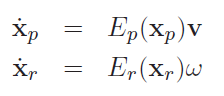
Forward kinematics gives you the ability to express

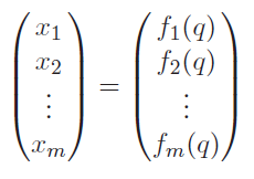
And you can derive the jacobian as an expression

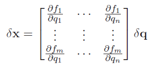
This tells us that if we knew $f(q)$, then we could easily compute this through simple derivatives. If we perform forward kinematic propagation, then this is usually the option we go for. However, we will also learn other ways of computing the Jacobian.

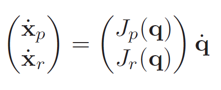
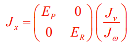
Because they take in the same $q$, you can express position and rotation together in a block matrix

Constructing Basic Jacobian

One issue we run into is that the $x_p$, and especially the $x_r$ is sensitive to representation. We want to get a Jacobian that tell us properties about the robot arm that is invariant to representation. This is the premise for the Basic Jacobian.

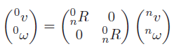
The Basic Jacobian $J_0$ is defined as

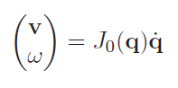
Where $v, \omega$ are linear and angular velocity vectors. You can define some $E_p$ that takes this $v$ into the desired representation, as well as some $E_r$ that takes the $\omega$ into the desired representation.

This is an abstract idea; in the next few sections, we will detail how we might compute this basic Jacobian.

Some cases of $E$

For position, you could have cartesian, cylindrical, or spherical. There may be others too

For rotation, you could have a ton of different things, including euler, quaternion, axis-angle, cosine angles

Linear and Angular Motion

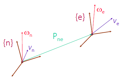
Let’s look at how we can describe linear and angular motion. Critically, we are interested in how we can describe motion in one frame WRT another frame. This will help us reformulate the Jacobian in a more general way.

First, some notation.

• $v_{P|A}$ denotes the linear velocity of point $P$ in frame $A$

Pure translation

Let’s say that we had a frame $A$ that was moving at velocity $v_{A|B}$ with respect to frame $B$. Then, let’s say that we had a point $P$ with velocity $v_{P|A}$. Then, as expected, we have

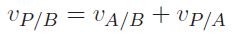
Which we can visualize nicely

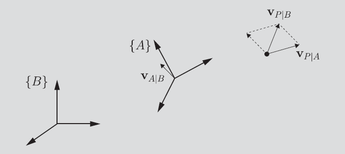
There is no angular velocity for obvious reasons.

Note that this is frameless, but if you wanted to express things in frames, you can just use the Homogenous transformation.

Pure rotation

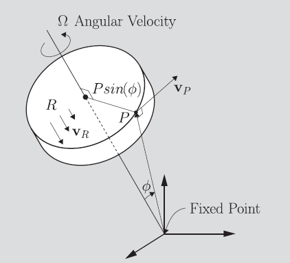
Let’s say that we had rotation around one axis. by definition, this is our angular velocity $\Omega$. But are we done? Is the linear velocity zero?

Your first thought might be that this doesn’t change linear velocity, but it’s actually a lot more nuanced. Unless you were sitting on the axis of rotation, the points in this frame of reference would actually be moving.

Specifically, you take the point $P$ and draw an orthogonal line to the axis of rotation. This forms a right triangle, with angle $\phi$ (for intuition, $\phi$ is zero if we are on the axis). Then, $P\sin(\phi)$ is the length of the shortest radius from the axis to $P$. Recall from physics that linear velocity is just $r\Omega$, so the linear velocity contribution of $P$ in rotation is $P\sin(\phi)||\Omega|| * \Omega^\perp$. Fortunately, there’s a nice, concise way of putting it:

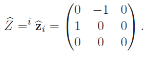
We can denote the cross product in matrix form, which we use the hat notation: $\Omega \times p = \hat{\Omega}p$.

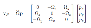
This is known as a skew-symmetric matrix. Again, this is a general property; we are not talking about frames yet.

Linear and angular motion

If you had concurrent liner and angular motion, what happens?

So for the angular velocity, the linear motion does not contribute to the angular velocity, so the angular velocity is still $\Omega$.

As for the linear velocity, you just add the linear component and the angular component.

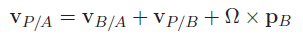
If you wanted it in the original base frame, then you would just need to make sure to convert everything into the same frame of reference before you performed the calculations

The rotational velocities are easier: they just add up.

Velocity Propagation

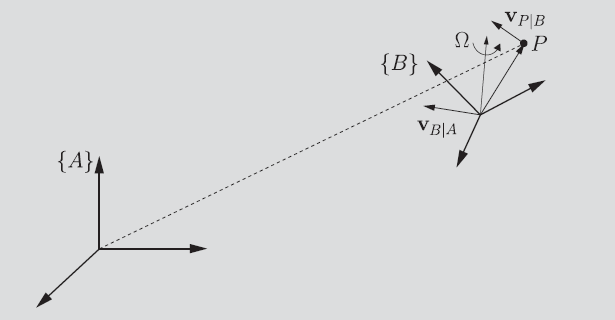
Now that we know how to express one frame’s velocity in terms of another frame, we are ready to start propagating velocities, just like we did with kinematics. The setup[ is as follows:

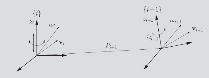
You have one frame with an existing linear and angular velocity, and you want to propagate it to the next frame, has a parameterized velocity $\Omega_{i+1} = \dot \theta_{i+1}z_{i+1}$ (i.e. joint speed times central axis).

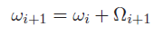
The rotational propagation is pretty easy. Angular rotation composes like vectors, so we have:

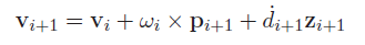
The linear velocity propagation is just adding the rotational component to the prismatic vertical component

Computing velocity propagation

These two equations don’t use any frames, but if you wanted frames, then you can just use the rotation matrix. Note that you don’t need to use the displacement anymore, because you’re concerned about the derivative.

It’s very important that you keep a consistent frame of reference as you are computing.

Explicit form Jacobian

We previously derived a way of propagating velocities without the Jacobian. We also previously mentioned the presence of the basic Jacobian. Now, let’s discuss how we might construct this basic Jacobian using the method of velocity propagation.

First, it helps to think about how prismatic and revolute velocities contribute to the linear and angular velocities.

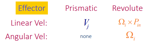
Contributions of prismatic and revolute joints

If you have a prismatic joint, then because the robot is rigid, the velocity simply propagates without any hiccups. The velocity contribution is $v_i = z_i \dot q_i$.

If you have a revolute joint, then the angular velocity also simply propagates with contribution $\Omega_i = z_i \dot q_i$.

The remaining problem is the linear contribution of the revolute joint. Well, it turns out that if we draw a vector $P_{in}$ from the current joint to the end-effector, then you’ve got that exact vector you need to compute the linear component of the angular velocity.

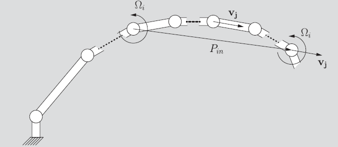
And that is just $\Omega_i \times P_{in}$.

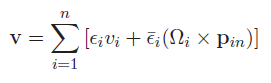
Creating the explicit expression

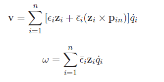
If we let $\epsilon_i$ be the indicator that the ith joint is prismatic, and $\bar{\epsilon}_i$ be the indicator that the ith joint is revolute, then the linear velocity is

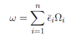
And the angular velocity is just

We can substitute the joint velocities into the equation to et

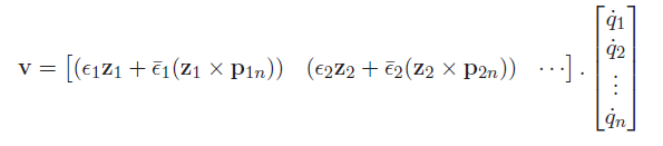
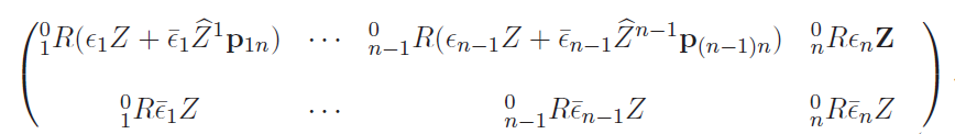
And we can write the linear motion as a matrix product

The rotational motion is a matrix product

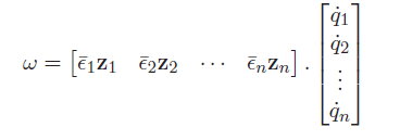
And this gets you the explicit Jacobian formulation. This matrix on the left hand sides for both expressions is the Jacobian!

Each $p_{kn}$ is the vector that points from joint $k$ to the last joint $n$.

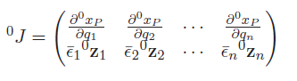
Actually doing this ⭐

The simplest way of computing a Jacobian is to find the $f(q)$ in a frame and then just take the derivatives and extract the z rotation axis. This is sufficient to get you the right Jacobian in that frame.

But what if we wanted to use the formula we derived? Well, we could compute all $z, p_{in}$ in the desired frame and take compute the cross product and stuff. Because cross products are agnostic to reference points, we can compute the cross product in the current frame. This is convenient because the cross product matrix becomes

And the expression becomes

Getting $p_{in}$

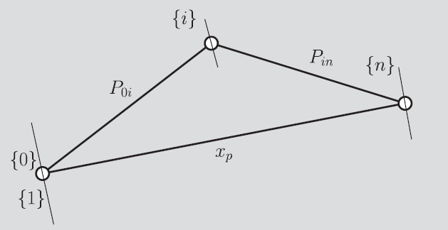
One thing we noticed about the previous derivation is that we needed $p_{in}$ which is the vector that points from joint $i$ to the end-effector. More precisely, we want $^ip_{in}$ to create our cross product. This requires access to $^i_nT$, which isn’t something that arises from kinematic propagation (because you typically compute $^0_kT$ for $k=1, …, n$. But there’s a pretty neat trick that gets around this problem. Just express

Now, $x_p$ is something that you know in frame 0 from position propagation, and $p_{0i}$ is something you also know from position propagation

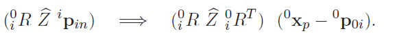
Unfortunately, however, this $p_{in}$ is in frame 0. But fortunately, you can just change the cross product operation to operate in frame zero:

Jacobian in different frames

If we want to change the frame of the Jacobian, you just need to transform the jacobians by a rotation

Cross product operator in different frames

Be warned: the cross product operator can’t be rotated like other vectors

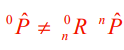
The math tells us that

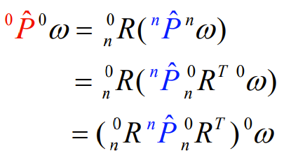
which effectively indicates that

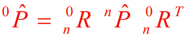
Intuitively, you move the vector into $n$ frame, do the operator, and translate it back.

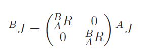
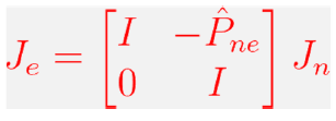
Jacobian at the End-Effector

Sometimes the end-effector is not the same place as the final frame. If you’re faced with this, you just need to consider one more linear velocity component

We add $\Omega_n \times P_{ne}$, but for the sake of simplicity, we actually subtract $P_{ne} \times \Omega_n$ so that we can write it as the following block matrix:

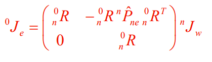
Alternatively, you could also modify the functions $f(q)$ and change the direct differentiation. The result is the same, and if you have the representaiton at hand, this may be easier. The end-effector equation with the frames becomes

Singularities

A kinematic singularity is a situation where we lose a degree of freedom. Recall that every joint adds a degree of freedom, but there are some situations where a particular configuration of joints makes you lose a degree. Also recall that a degree of freedom doesn’t necessarily always mean motion in one direction.

We always measure singularities from the end-effector point of view because it’s often much easier to do that.

Representative examples

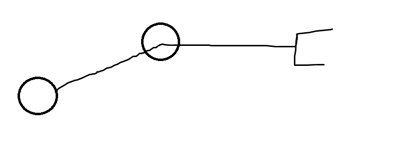
Consider this joint setup. At this configuration, there are still two degrees of freedom.

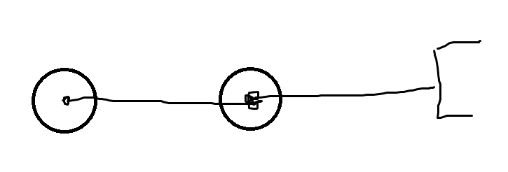
But at this configuration, we only have one degree of freedom in the end-effector. We lose the ability to move left and right. A good way of thinking about things is to imagine trying to perturb the different axial directions as you approach the singularity. One direction should vanish.

A good rule of thumb: if we wiggle each joint, how does everything else wiggle? Existing joint limits are not singularities.

In general, it’s ok if you have correlated motion, i.e. it’s ok if you move multiple axes at once; that’s still having the freedom to move. When you actually vanish, that’s when you have a singularity.

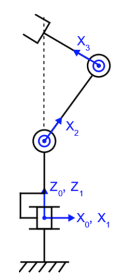
This is a more complicated example, but we can see that in this configuration, we lose the ability to move in and out of the page. We can still move up and down, and left and right.

Formalization of singularity

Formally, the Jacobian tells us how some $x$ changes as you vary $q$. During a singularity, it means that you can’t reach a certain way that $x$ changes. This should be ringing some alarm bells in your head about matrix properties.

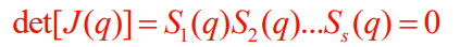
If the jacobian is square, then if we are singular, then $\det(J) = 0$. The determinant is the same regardless of measurement frames. Often, you can write out a determinant as a product of numbers, and this tells us the different singular configurations

For a review on how to compute the determinant of a 3x3 matrix, see the math review