Physics background

• Moment of inertia is the integral of the mass with radius squared

• The “torque” of a prismatic joint is just acceleration; it has different units.

• Product rule works with cross products

• For a vector quantity $q$, we assume $\dot q$ is the time derivative

Math review

When we have $d/dt \cos(\theta)$, we get $-\sin(\theta)\dot \theta$. Make sure that you follow the chain rule completely.

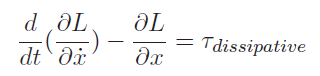
Lagrange equation

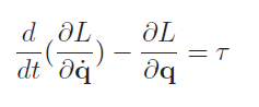
We let the Lagrange $L = K - V$. IT turns out that this formulation allows for a critical result.

This critical result is derivable from Newton’s equations and a lot of math.

In other words, the force into the system can be purely modeled in a differential equation. If there is no force, then the Lagrange equation’s right hand side is zero. This is critical because it allows us to describe a complicated system through time

For a degenerate example, if we are working with a particle in the z direction, we have $L = 1/2 mv^2 - mgx$. When left without any perturbing forces, we have $ma - mg = 0$, meaning that $a = g$. This means that the particle accelerates downwards, as desired! But we can move this to any arbitrary system with high complexity. We just need to formulate the Lagrange, and solve the differential equation.

Why do we care about dynamics?

Dynamics is all about finding the forces, velocities, and accelerations on each link of a robot arm. It’s not as easy as you might think: forces on one joint will propagate to all other joints in a process known as “inertial coupling.”

The two approaches

The newton-euler algorithm derives velocities, acclerations, and dynamic forces through a forward propagation, and then backpropagates through the structure to find moments. This is rather complicated and we tend not to use this formulation.

The Lagrange formulation relies on energy and involves the mass matrix explicitly.

Both ways of understanding dynamics yields the same final equation:

These are called the equations of motion . An equation of motion is a differential equation. When solved, it allows you to compute the exact paths. Or, you can potentially solve the equation one way to derive the accelerations on the joints given the velocities and the positions, etc. There’s a lot we can do, and we’ll get to them later.

Newton-Euler

There are two parts of this formulation. Newton’s equation tells us about linear motion, and Euler’s equation tells us about angular momentum and inertial tensor.

Linear and angular momentum relationship to force, moment

Let’s start with the motion of a single point.

Newton’s law tells us that $F = ma$, which means that $\frac{d}{dt}(mv) = F$. Turns out, $mv$ is momentum, so you can understand force as a change in momentum (shouldn’t be news to you).

Angular momentum is a bit more complicated, but it’s the same as anything angular that we’ve done so far. Angular momentum is just $p\times mv$, which is the rotational analog of linear momentum. We take the derivative and apply the product rule to get

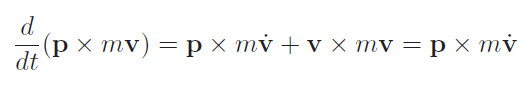
which is the applied moment $N$.

Euler Equation

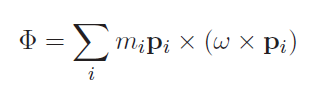
We extend our analysis from a single point to a collection of points. Let’s compute the angular momentum of any rigid body. We start with some knowns

• Linear velocity of any point is $\omega \times p_i$

• Angular momentum is $p\times mv$

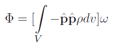
Putting this together, we get that the angular momentum $\Phi$ of any rigid body is

The integral version is

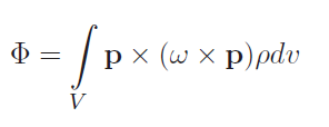
where $\rho$ is density. This is a formulation that gives the angular momentum of any object.

We can replace the cross product with the operator to get

Now, the quantity inside the bracket is a matrix, and it is called the inertial tensor which we denote with an $I$. So, we can still write the angular momentum of the whole rigid body as

As expected, when we take the time derivative, we get the moment $N$

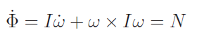
Notice that this gets you an equation of motion, relating applied force to acceleration.

Inertial tensor

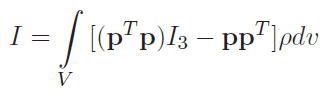
As we hinted at, the inertial tensor is an integral defined as

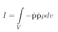
Now this is the 3d analog of a MOI calculation which is $\int r^2 dm$. We can write the quantity $-\hat{p}\hat{p}$ as

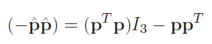
so the inertial tensor can be rewritten as

If $p$ uses a cartesian representation, the matrix is

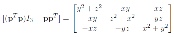
If you want, you can integrate each component separately. The on-diagonal components are called moments of inertia, and the off-diagonal components are called products of inertia. These products of inertia tell us something interesting: there is typically some coupling between the different axes of rotation.

• Actually calculating the intertial tensor

  Use the parameterization $p = [x, y, z]$ and you’ll get a matrix of integrals. Compute the integral of each component (nine integrals), and you might find some symmetry too.

MOI, POI

The inertial tensor is a symmetric matrix with some interesting properties.

The MOI is the diagonal components of the inertial tensor. This represents the inertias that you’ll encounter when you rotate the object along the fixed axes. By definition, they must be positive

The POI are the off-diagonal components of the tensor, which can be positive or negative. Their actual values are less meaningful, but they can tell us something. Namely, they are non-zero only if the mass is distributed unevenly around the axis. The xz direction looks at imbalance in the xz plane, the xy direction in the xy plane, etc. This happens if you offset the reference axes from the center of mass.

This tells us something interesting: there is definitely some point on any object that yields a diagonal inertial tensor. The parallel axis theorem tells you how the off-diagonals change when you move that axis around.

Parallel Axis Theorem

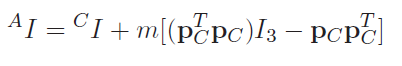
Turns out, you can just find the inertial tensor at the center of mass and translate it into a new frame.

If the frame is parallel to the center of mass (i.e. just one translation), then we get

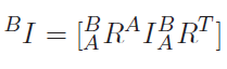
And if there is some rotation, we use the old trick of going in and out of that space

Lagrange Formulation

The Lagrangian is the difference between kinetic and potential energy of mechanism: $L = K - V$. This $V$ is a function of $q$ only, and this $K$ is a function of $q, \dot q$. We discuss this formulation above.

Logistically, you let $\dot q$ be the variable (for example, it could be $v$), you take the derivative, and then you treat this $\dot q$ as a derivative again and take the derivative through time. We’ll open up an example later.

And because potential energy only depends on $q$, we can reformulate it as

The term $dV/dq$ is a gravity vector and should be pretty easy to derive. The first two terms are inertial forces. Together, this forms an equation of motion.

Inertial Components

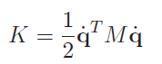
We can express the kinetic energy as a quadratic form with the mass matrix (see below sections)

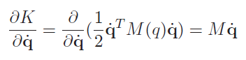
If you choose to take the derivative WRT $\dot q$, we get

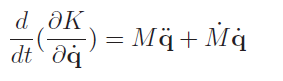
And then we take the derivative through time using the product rule (note that it is not just $M \ddot q$)

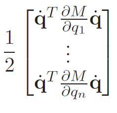
As for $\partial K/\partial q$, we realize that the only thing dependent on $q$ is the mass matrix. This gets you a gradient of the form

Putting it all together, we get that the equation of motion is of the following form:

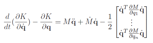
which we can rewrite into $M \ddot q + V(q, \dot q)$ where the last two terms are grouped together.

Writing out kinetic energy in explicit form

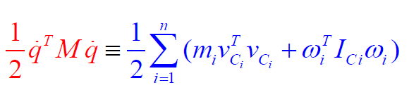
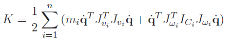
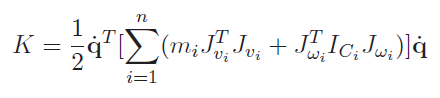
What if you don’t have the mass matrix? We’ll talk about the mass matrix below. But you can also assemble it iteratively. First, note that $K = \frac{1}{2}\dot q^T M \dot q$, but because energy is a scalar, we can also just say that the energy is the sum of the energies at each joint.

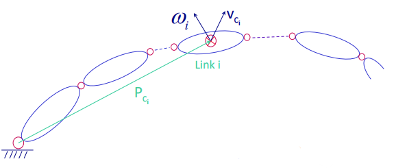
At each joint, the kinetic energy is just the sum of the linear and the angular velocities, which can be expressed as the following:

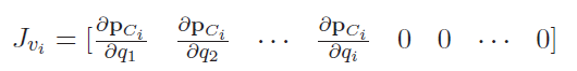
which means that you can build up the kinetic energy function iteratively. The velocities can be derived from the joint velocities through the Jacobian, so we get

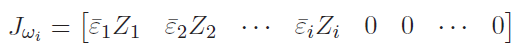
Now, what are these Jacobians? Well, the velocity of any center of mass does not depend on any joints afterwards! So the Jacobians are zeros for anything after that joint. Otherwise, we just take the derivative of the COM functions of q

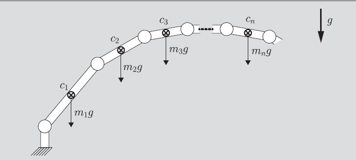
Gravity Component

To complete the Lagrange formula, we need the gravity vector and $dV/dq$. It helps to realize that we can add the potential of each COG

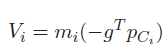
The potential energy is really easy to formulate. We can just have

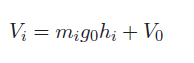
where $h$ is the height of the center of gravity. This is also the projection of the gravity force along the direction.

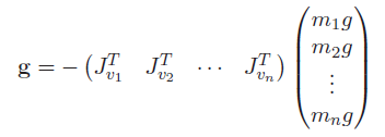
If we take the gradient of this expression WRT $q$, it’s very similar to computing the Jacobian. Indeed, you’ll get the form

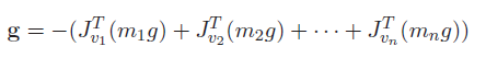
Here’s another way of interpreting the gravity component. Recall that the $G$ is in units of torque. But we already know how to calculate static torque! Just use the fact that $\tau = J^TF$ and add up the individual torques

This actually gets you the exact same formulation

Mass Matrix

The mass matrix tells us how different joints influence different torques. In a static setting, $M\ddot q = \tau$. Of course, this changes in the dynamic setting, but this tells us that there may be an interdependence between joints, held by the off-diagonal terms. The Lagrange formulation used this $M$ in the motion equations. Now, let’s talk about how we might compute it explicitly.

• Example

  Let’s try to understand the mass matrix with an example. We start with a simple, two-joint system

  

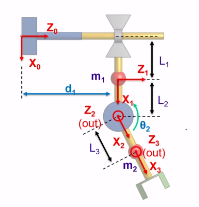
  Let’s assume that we are operating in a vacuum and nothing is moving. Therefore, $M\ddot q = \tau$. But what is $M$?

  

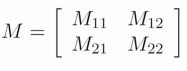
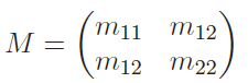
  As it turns out (now this isn’t obvious), the mass matrix is

  

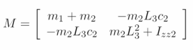
  where the $I_{zz2}$ component is the existing MOI on the joint itself. We will discuss the mass matrix in more detail later.

The mass matrix is symmetric, which is interesting. This tells us that if one joint influences another joint, then the other joint should also influence the original joint in the same way. The diagonal components of the mass matrix must be positive because of Newton’s law. The off-diagonal components can be negative because it just says that one torque has a negating effect on the other joint.

Explicit formulation

Previously, we asserted that the kinetic energy can be expressed as a summation.

We can just rearrange this to become

which indicates that

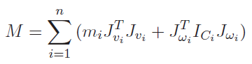
This gives us everything we need to explicitly compute a mass matrix. Make sure that the $J_{\omega_i}$ and the $I_{C_i}$ are in the same reference frame. This $J_{\omega}$ need not to be in the same frame as $J_v$. Indeed, usually $J_v$ is best represented in frame 0, while Jw needs to be in the frame of the inertial tensor. Different $J_v$ in the summation can also have different frames of reference.

Centrifugal and Coriolis Forces

In the Lagrange formulation, we had the $v$ component as follows.

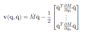
This is actually a sum of centrifugal and Coriolis forces. Let’s dive deeper into what we mean.

Cristofel Symbols

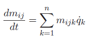
The mass matrix element $m_{ij}$ could depend on $q$. We denote the partial derivative WRT $q_k$ as the (slightly confusing)

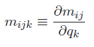
We the Christoffel symbol defines

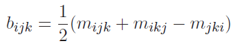
This sounds weird, but we’ll see why it exists in a second.

We also note that $\dot m_{ij}$ can be computed by the chain rule

Building from a 2d example

We want to create a general case for this $V(q, \dot q)$, but it actually helps to start from a 2d example

which gets us

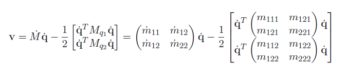
using the formulation that we previously discussed. If we multiply everything out, we see that there’s actually a special structure

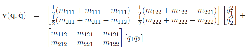
where $[\dot q_1 \dot q_2]$ is a single number. This is where the previously-defined Christoffel symbols come in: we can replace this messy setup with. This gets you

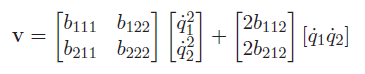
and this is precisely the centrifugal and Coriolis contributions. This first matrix is related to the squared velocities, and so we have the Centrifugal forces. The second matrix is the Coriolis contrigution.

General case

We can this $v(q, \dot q)$ as the follows:

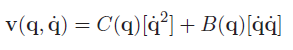
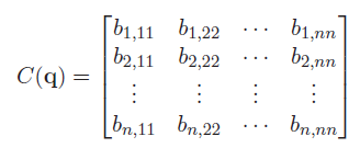
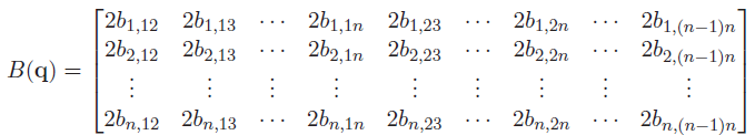
where $\dot q^2$ is just element-wise squareing, and $\dot q \dot q$ is the pairwise products of all joint velocities of size $(n -1)n/2$

The general form of the matrix is

Building Intuition

Of course, the question becomes this: we’re seeing a lot of math, but what does it actually mean? Well, let’s consider this arm and a closed-form derivation.

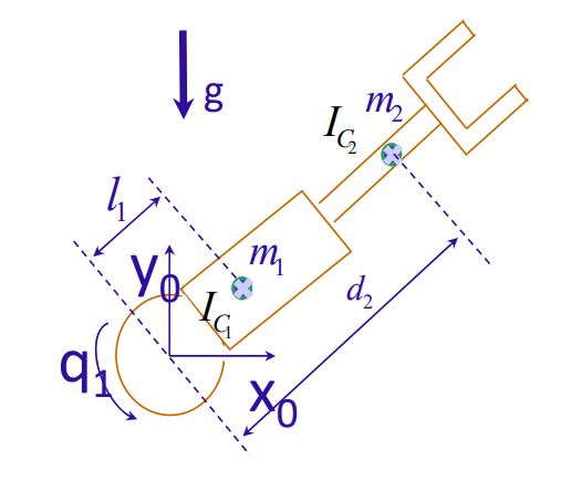
Deriving mass matrix

We start by writing the mass matrix in explicit form:

And we can derive each Jacobian because we have the explicit position parameterization

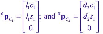
which yields the Jacobians

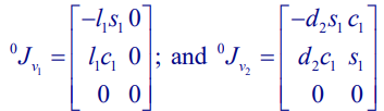
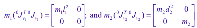
Now, if we just shove everything into the formula, we get

We can compute the angular jacobians, which have a very simple form

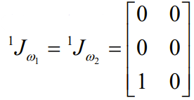
Which gives us the following products

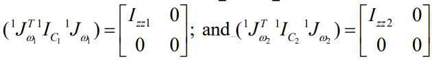
And when we finally put everything together, we get the mass matrix

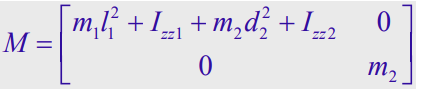
This tells us that the two joints are not coupled, which makes sense.

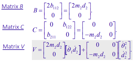
Coriolis vector

If we follow the formula described above, we get the following format:

Gravity vector

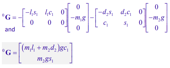
We can just compose all of the forces on each joint,

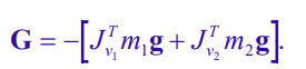
We use frame 0 to be convenient. After doing this composition, we get

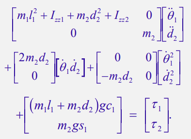
Putting it all together

The equations of motion look complicated, but it’s completely closed form. We can relate desired velocities and accelerations with joint torques

Debrief: the general steps

1. Compute the Jacobians for each joint

2. Use it to find the mass matrix

3. Use the mass matrix to compute $V$

4. Compute the gravity vector separately

5. Add everything together