Practical Tips and Tricks

DH tips and tricks

Remember that you need to align the x axis to point at the next joint, and you do this by rotating the $z$.

Ordering of rotation

Follow the order of rotations as specified by the joints; failure to do so can yield a bogus result

Importance of $\theta, d$

These $\theta, d$ are free parameters, meaning that they will be used to make the robot legal. This will be painfully apparent if you have a world frame whose $x$ doesn’t line up with the next joint. This is where the $\theta$ comes in.

If you are given axes → Derive DH parameters

If you are given axes, the derivation should be simple. Just propagate the frames using the four step method. At a given point $i$:

1. Using previous $x_{i-1}$, find translation from the previous frame to the new frame along axis $x_{i-1}$. Note that this may NOT be the final location of the frame because we have another translation later

2. Using previous $x_{i-1}$, find rotation along this axis that takes $z_{i-1}$ to $z_i$. Often, this is some multiple of 90 degrees. Remember to use right hand rules

3. Using the current $z_i$, find the rotation along $z_i$ that takes $x_{i-1}$ to $x_i$. Rembmer right hand rule. Also remember that prismatic joints may have a twist.

4. Using current $z_i$, find the translation along $z_i$ that takes us from where we are, to the next frame. Remember that revolute joints may have a displacement.

If done right, you should be able to traverse the whole robot through these cyclical sequence of translations and rotations. Note that the first two steps are interchaneable, and so are the last two steps.

If you are given DH parameter → derive axes

This is actually the more tricky variant of this problem because it requires you to work backwards. There’s a degree of dynamic problem solving in place, although there are some tips and tricks.

• Prismatic joints are annoying because technically, you can place the next frame anywhere along the line specified by $z_i$. You may have to edit your response later

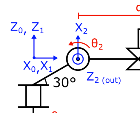
• Revolute joints can be tricky! Don’t assume that $\theta$ is at zero in the current configuration; in fact, it may definitely not be zero

• Don’t get fooled by angles! In the example below, 30 degrees contributes to the offset $a$, but it the angle of the joint is actually 90 degrees

The general method is to build up the axes systematically. If you do it correctly, everything will be self-consistent. Building up the axes sysematically means doing the following:

1. Propagate the new origin using $a_{i-1}$, the previous frame, and the previous $x_{i-1}$.

2. Find the new $z_i$ using $\alpha_{i-1}$ and the previous $z_{i-1}$

3. Find the new $x_i$ using $d_i$ and $\theta_i$

If you are given nothing

If you start from scratch, know that you can define the axes quite arbitraily. So I would recommend doing the following

1. Assign axes systematically without worrying about the angles or the lengths (recall: if overlapping $z$, pick the $x$ that yields positive rotation $\alpha$
   1. Start with $z$ first, because their axis is known (they must be through a revolute joint and prismatic joint)
   2. $x$ always points to the next joint (if it’s not, you’re doing something wrong). Tiebreaker: if the frames overlap, pick $x$ that creates positive angles.

2. Label your active angles and shifts. See above in how to derive DH parameters from an axis set.

Remember that an angle $\theta$ doesn’t influence any future links, so you won’t have to worry about any weird dependencies. If you are worrying about it, then you’re doing something wrong.

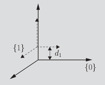
Common confusion is mixing up $a_{i-1}$ with $d_i$. The first one is along the x axis of the previous frame, which is often zero. The second one is along the z axis of the current frame.

Links

A link connects two joints. A joint can be revolute around the central axis, or it can be prismatic that moves along that central axis (note that it doesn’t affect the link itself, which is always rigid).

There are few properties we need to pay attention to.

Between two links

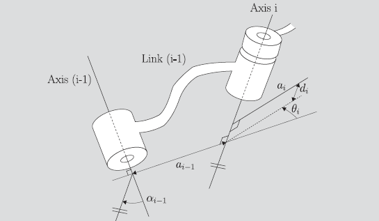
The two links have their own axes. With two axes, you can narrow down a common normal.

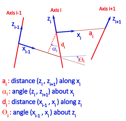
The link length, or $a_{i-1}$ in the diagram, is the length along the common normal from axis $i-1$ to axis $i$. Note that the link may be weirdly shaped, but all you care about is this common normal. The common normal is the shortest distance between these axes.

If project the axis $i$ onto axis $i-1$ along the common normal, you’ll get an angle denoted as $\alpha_{i-1}$ above, and it references the link twist. Note that this is the same angle you’d have to twist axis $i-1$ along the common normal to get the joints to align. This also latches onto the theme of all rotations being represented by an axis and an angle.

Two special cases exist:

• First, if the links are overlapping, then the link length is 0.

• Second, if the links are parallel, then the link twist is 0.

Connecting links together (DH Parameters)

So we saw how link length and link twist are important parameters for a link. Now, this is a stationary property that doesn’t change with joint angle. So how does joint angle play into it?

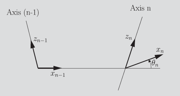
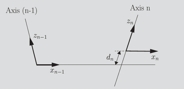
Well, if we look at the next link, we realize that the angle between our current common normal and the next common normal is determined by $\theta_i$. And the vertical offsets between the common normals are determined by $d_i$, the prismatic offset. In revolute joints, $\theta_i$ changes but not $d_i$. Vice versa for prismatic joints. However, it may be the case that revolute joints have a constant offset (because of the hardware), and prismatic joints have a constant rotation. This must be considered in the equations.

These four parameters: $a_i, \alpha_i, \theta_i, d_i$ tell us how two links behave. These are known as the Denavit-Hartenberg parameters. You can imagine $a, \alpha$ telling us how the link works, and $\theta, d$ telling us how to orient the next link.

First and last links

With our four parameters, we can define $\alpha, a$ for $i = 1, 2, 3, …, n-1$. But the first and last links are really weird. The first link is base → first joint, and the last link is last joint → end-effector tip.

You could specify the base as something different than the first joint, which would mean that you have non-zero $\alpha, a$. However, conventionally we assume that the base overlaps with the first joint, which means that the only non-zero property is $\theta_0$ or $d_0$.

For the last link, we know that there is no extra joint, so $d_n, \theta_n$ must be 0. For simplicty, we also assume that the last joint is the end-effector, which means that $\alpha_n, a_n = 0$ as well. This is just for simplicity.

Notation

Rotational joints are denoted as “spools”. The spools rotate as if you had a pin in the hole that goes through the spool. Primatic joints are denoted as diamonds. They move along the axis that the diamonds pinch.

Attaching Frames to links

In general, for each joint, three of the Denavit-Hartenberg parameters will be fixed and one will be variable.

We can do this by using a fixed convention. First, let’s define the point of the frame of axis $i-1$ as the intersection of the shared normal $a_{i-1}$ and the axis vector.

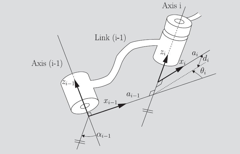
Direction convention

Let $X$ point along the common normal to the next axis. Let $Z$ point in the direction of the axis. The $Z$ direction is actually arbitrary, but it influences how you define $Y$ and the positivity of the angle.

If the axes intersect (like with a sphere joint), you will need to make a choice on the direction that $X$ points. Choose the direction such that the angle from axis $i$ to $i+1$ is positive.

Now, note that this $\alpha$ is defined as the direction you would need to rotate axis $i-1$ to align with axis $i$. This is consistent with using the right hand rule around axis $X$.

First and last links

The first and last links are also tricky. As we mentioned above, we should try to set the base as close to the reference frame as possible. In revolute joints, that means setting $a_0 = \alpha_0 = d_1 = 0$, meaning that when $\theta = 0$, the base frame is the first frame. Simialrlly with prismatic joints, we want to pick something where $a_0 = \alpha_0 = \theta_1 = 0$.

And the last link math is similar; make sure that you set zero offset except for what the joint does. This corresponds to having the last joint be the end-effector.

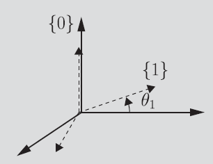
Example: RRR

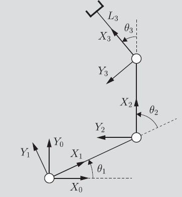
If we consider a planar robot with 3 joints, we can see how the parameters come together. You can see how frame 0 is the base, and how frame 1 aligns with frame 0 when $\theta = 0$. Because all joints are planar, the $\alpha = 0$ for all $\alpha$, and the $a$ is just the length of the link. So this is one of the simpler setups.

Good diagram

Propagation of Frames

Now the big question is this: given the DH parameters for the arm, can we derive the different frames?

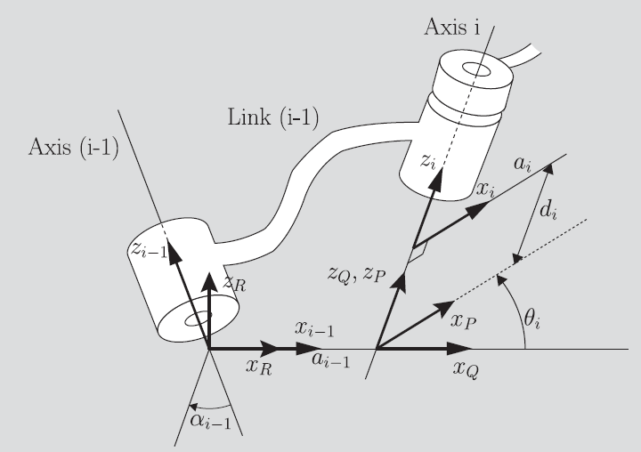
The trick is that each of the DH parameters specify a particular transformation, and the composition is actually really simple. From frame $i-1$, you want to…

1. apply a rotation matrix to align the two joints. By construction, this means that you rotate around the x axis by $\alpha$ degrees

2. apply a translation to move joint $i-1$ to joint $i$. Note that because you’re already aligned on the common normal, so you just have to translate the $x$

3. Apply a rotation (if needed) that represents the rotation of this next joint. Because you’re already aligned this is just a rotation around z

4. Apply a translation (if needed) that represents the motion of the prismatic joint. Because you’re already aligned, this is just a translation with $z$.

This can be written as

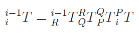
Which you can imagine as rotating the previous joint to align with the current one. Then, moving this joint to the current one. These are actions on the $x_{i-1}$. Then, you rotate and translate around $z_i$, which creates your current $x_i$. Remember: first create the z from the x, then the x from the z.

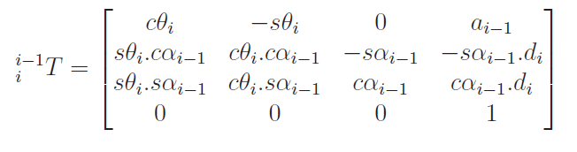
And here’s what the operator looks like

• The final homogenous matrix

  

Kinematics of Manipulators

Once you know how to bring us from one frame to another, you can map joint angles to positions and rotations!

Direct Kinematics

This brings us to the concept of direct kinematics, which is mapping joint space coordinates to task space.