Proof tips

• Uniform continuity: to dissapprove, use a pair of sequences. To prove, show that $\delta_\epsilon$ doesn’t depend on $x$, or show that it is bounded, or show standard continuity and use the continuity theory

• Closed and bounded: immediately think about some sort of sequence and use BW to make a subsequence
  • somehow exploit that all $\lim x_n \in S$ as well

• Continuous: always use $\lim f(x_n) = f(\lim x_n)$.

• feel free to use a sequence to define limiting behavior of functions; this is actually quite helpful at times

• You can show that something is not uniformly convergent if you can find a cauchy $s_n$ such that $f(s_n)$ is not cauchy.

• Anchor technique: if you want to show two moving points like $x, y$ and you have some fact about limiting to an anchor point, use trianglie inequality to set up two point limits (to some anchor point) and relate this to the $x, y$ together.

• The tricky part is that sometimes you get weird behavior with functions. Just because $x_n$ converges doesn’t mean that $f(x_n)$ converges. A good example is $x_n = 1/n$ and $f(x) = \sin(1/x)$. We need to show this
  • it helps to consider $y_n = f(x_n)$ as a completely different sequence

• Raising floor trick: if you want to show that a function $a_n$ eventually surpasses $c_n$ and you also know that $b_n$ appraoches $c_n$, if you can find a relationship between $a_n$ to $b_n$ (like $a_n \geq b_n$) then as the “floor” rises, you can eventually show that $a_n > c_n$. This is a common trick and if you have limit behavior, this is definitely one thing to look out for.

• Uniform continuity: show continuity and then show that $\delta_\epsilon$ doesn’t depend on $x, y$.

Functions

Definition 🐧

A function is something that maps between elements of $A$ to elements of $B$. These sets can be finite or infinite. One input maps to only one output (i.e. the vertical line test)

Cardinality 🐧

The cardinality of a set is the number of elements in it, typically denoted with $|A|$.

A countable infinity is just defined as $|\mathbb{N}|$. There are an infinite number of uncountable infinities. Anything is countably infinite if you can make a bijection between $\mathbb{N}$ and the set.

Injective, surjective, bijective 🐧

An injective function has all $a\neq b → f(a) \neq f(b)$, i.e. the horizontal line test. A good way of proving injectivity is to have $f(a) = f(b)$ and showing that $a = b$.

A surjective function has the following: for all $b \in B$, there exists some $a \in A$ such that $f(a) = b$. There might be more than one, of course. A good proof trick is to pick a random $b$ and show that an $a$ exists.

A bijective function is both injective and surjective. This means for all $b \in B$, there exists one and only one $a \in A$ such that $f(a) = b$.

Finite results from injective, surjective, bijective 🚀

If $A, B$ are finite, then if $f$ is surjective, then $|B| \leq |A|$.

• proof (contradiction + function definition)

  by contradiction. If $|B| > |A|$, then by the pidgenhole principle, there exists some $b_1, b_2 \in B$ such that $f(a_k) = b_1, b_2$, which violates the funciton definition.

If $A, B$ are finite, then if $f$ is injective, then $|A| \leq |B|$

• proof (contradiction + function definition)

  If $|A| > |B|$, then by the pidgenhole principle, there must be some $a_1, a_2 \in A$ such that $f(a_1) = f(a_2) \in B$, which violates injectivity.

Key result: if $A, B$ are finite, if $f$ is bijective, then $|A| = |B|$.

Weird results for infinity 🚀

For infinite sets, these rules don’t hold. For example, you can make a bijective mappings between $\mathbb{N}$ and $2\mathbb{N}$, but the number of elements is less is the second set. But, of course, we have a bit of a circular definition for cardinality in the infinite domain. Because we can make a bijective mapping between $N, 2N$, we conclude that they have the same cardinality.

Function rules 🔨

• For any set $S$ and function $f$, the set $f(S)$ exists.

• For any set $S$ and the function $f$, the set $f^{-1}(S)$ exists. This is a little unintuitive, because the pointwise inverse might not exist. But you read $f^{-1}(S)$ as “the set of all values $x$ such that $f(x) \in S$”, and this is valid
  • invertible functions form a bijection

• If as set $S$ is open, then $f^{-1}(S)$ is also open, if it’s continuous. Vice versa. This is not true for forward fuctions. If $S$ is open, consider $f(x) = 1$. This is a closed $f(S)$.

Limits of Functions

Delta Epsilon Definition 🐧

A limit of a function $\lim_{x → x_0}f(x)$ is defined to be $l$ if, for all $\epsilon > 0$, we have $|f(x) - x_0| < \epsilon$ for all $x \in (x_0 - \delta, x_0 + \delta)$ for some $\delta > 0$. Graphically, this looks like the following

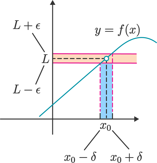
It’s actually quite similar to the epsilon definition for a sequence. The only difference is that we must bound $x$ on both sides, and we must use an interval because there is no notion of natural number indexes.

As a key note, we need $\delta > 0$. If $\delta = 0$, then we are considering the function evalutaed at $x_0$, and in limits, we care about the neighboring behavior, NOT the actual behavior at $x_0$ as sometimes it can be undefined, like $\sin(x)/ x$ for $x = 0$

Showing limits 🔨

Just like in sequences, you need to take an arbitrary $\epsilon$ and show that you can find a $\delta_\epsilon$ that satisfies the limit definition.

• Example

  Prove that $\lim_{x → 0} x\cos(x) = 0$. We start with $|x\cos(x) - 0| = |x||\cos(x)|$, and we want to define some $\delta$ such that all $|x - 0| < \delta$ satisfy $|x \cos(x)| < \epsilon$.

  We note that $|\cos(x)| \leq 1$, so $|x||\cos(x)| < |x|$.

  So, if we let $\delta = \epsilon$, we have $|x - 0| = |x| < \epsilon$, which means that $|x||\cos(x)| < \epsilon$ as desired.

Continuity

The definition 🐧

A function is continuous at $x_0$ if and only if

We say that a function is continuous as a whole if for all $x \in dom(f)$, we have that the function is continuous at $x$.

• Alternative definition (with sequences)

  You can also skip the definition of a limit of a function and use the definition of sequences directly, such that you make a sequence $x_n$ with $\lim x_n = x_0$, and then you apply the function on it. You need to show that all sequences with this property will satisfy this

Showing continuity 🔨

You can show it through the formal definition, i.e. find a $\delta$ such that $|x - x_0| < \delta$ mean that $|f(x) - f(x_0)| < \epsilon$.

You can also use limit laws to compute $\lim f(x)$ and show that it becomes $f(x_0)$.

Showing discontinuity 🔨

You just need to compute the limit at $x_0$ and show that it doesn’t converge to $f(x_0)$ for some $x_0$.

Continuity theorems

If $f$ is continuous, then $|f|$ and $kf$ are continuous, where $k$ is a finiite multiplier

• Proof

  $|f|$: if $|f(x) - f(x_0)| < \epsilon$ for all $|x - x_0| < \delta_\epsilon$, , consider $||f(x)| - |f(x_0)||$. We can actually show that $||f(x)| - |f(x_0)|| < |f(x) - f(x_0)|$, so we are done.

  $kf$: Consider $|kf(x) - kf(x_0)| = |k||f(x) - f(x_0)|$. We know that $|f(x) - f(x_0)|< \epsilon / |k|$, so we are done.

If $g, f$ is continuous, then $g + f, g * f, f/ g$ is continuous at $x_0$. ( the last one only if $g(x_0) \neq 0$.

• Proof

  This is just limit theorems. We know that limits can be split through sums, products, and divisions.

If $g$ is continuous at $f(x_0)$ and $f$ is continuous at $x_0$, then $g\circ f$ is continuous

• Proof

  We have that $\lim f(x) = f(x_0)$, and we have that $g$ is continuous at $f(x_0)$, which means that $\lim_{k →. f(x_0)}g(k) = g(f(x_0))$. We know that $\lim_{k→f(x_0)} g(k) = \lim_{x → x_0}g(f(x))$, so we have $\lim_{x →x_0}g(f(x)) = g(f(x_0))$ as desired

Local and Global properties 🐧

A local property of a function is something that only concerns some $x \in (x - \sigma, x + \sigma)$ for some finite $\sigma$. Examples of local properties include

• the value of a function (duh)

• continuity at a point

• limit of a function

• derivative at a point

A global property depends on the whole function, unbounded. Some examples include

• the max/min of a function

• the integral of a function

Implications of continuity

Boundedness of continuous functions 🚀

Claim: if $f$ is continuous on $[a, b]$, then $f(x)$ is bounded on $[a, b]$. This $[a, b]$ must be bounded and closed; you can replace it with any bounded and closed $S$ if you want.

• Counterexamples

  Say you had $f(x) = 1/x$ and take the interval $(0, 1]$. This $f$ is not bounded!

  Say that you had $f(x)$ and take the interval $[0, \infty)$. This $f$ is not bounded!

• Proof (contradiction)

  We approach this by contradiction. Suppose that $f$ is not bounded. Then, by definition, for any $M$, there must exist some $x_m$ where $|f(x_m)| > M$. Now, consider making a sequence $x_1, x_2... \in [a, b]$, where each $x_k$ has the property $|f(x_k)| > k$.

  Now, as a key fact, this sequence need not converge. However, by the Boisano-Weirerstrauss theorem, because $[a, b]$ is a compact set, we have that there exists a subsequence $x_{b_k}$ where $\lim x_{b_k} = x \in [a, b]$.

  Now, because $f$ is continuous, we have $\lim f(x_{b_k}) = f(\lim x_{b_k}) = f(x)$. Now, the problem is that we were suppose to show that $\lim f(x_{b_k})$ diverged to $\infty$, but we showed that it is equal to $f(x), x \in [a, b]$. The function maps to the real domain, so this is a contradiction.

Because we have shown that $f$ is bounded, we have shown that $\inf(f), \sup(f)$ exists. Now, we will show that we actually reach the infimum and supremums

Existence of maxima and minima 🚀

Claim: for any interval $[a, b]$, there exists $x_0, x_1$ such that $f(x_0) \leq f(x) \leq f(x_1)$.

• Counterexamples

  If we have an open interval $(0, 1]$, consider $f(x) = x$. In this case, $\inf(f) = 0$, but this is never reached.

  If we have an unbounded interval $[1, \infty)$, consider $f(x) = 1/x$. In this case, $\inf(f) = 0$, but this is never reached.

• Proof (definition of inf, sup)

  Let’s look at finding $x_0$. Let $S = \{y : y = f(x), x \in [a, b]\}$. Now, given any $m > 0$, we know that there exists some $y_m \in S$ such that $\inf(S) \leq y_m \leq \inf(S) + 1/m$. As such, there must exist some $x_m$ such that $\inf(S) \leq f(x_m) \leq \inf(S) + 1/m$.

  The sequence $\{x_m\}$ may not be convergent. Consider an extreme example where there are two minima of $f$, and $x_m$ oscillates bewteen the two minima points. This is valid because the inequality is satisfied, and $y_m = f(x_m)$ most certainly converges, but $x_m$ does not.

  Even so, we know from the above (sandwich theorem) that $\lim f(x_m) = \inf(S)$. Now, because we are in a closed and bounded set, we know that we can construct a subsequence $x_{b_m}$ such that $\lim x_{b_m} = \tilde x$. Now, we envoke the continuity definitions, and we can say that $\lim f(x_{b_m}) = f(\lim x_{b_m}) = f(\tilde x)$. Now, here’s the tricky realization. We know that $y_m$ converges to $\inf(S)$, so all subsequences $y_{b_m} = f(x_{b_m})$ converges to $\inf(S)$.

  ☝

  The key difficult thing to wrap your head around is that the image is a convergent sequence but the preimage is not. You need to manipulate the preimage using the BW theorem, and you get a subsequence of the image, which you know converges.

  The existence of a maximum is the same sort of proof.

Intermediate Value Theorem 🚀

Claim: let $m$ be the minimum and $M$ be the maximum that a function takes on in $[a, b]$. For any $m < y_0 < M$, there must exist a $x_0$ such that $y_0 = f(x_0)$, if $f$ is continuous.

• Proof (contradiction; tricky!)

  Like before, we want to find this $x_0$. Let’s define a set $S = \{x : f(x) \geq y_0\}$. We claim that $f(\inf(S)) = y_0$. We show this by contradiction. Let $i = \inf(S)$. Intuitively, we’re saying that we can find $x_0$ the first time the function becomes $y_0$. There may be more $x$, but we just need to show that one exists.

  Suppose that $f(i) > y_0$. Therefore, because $f$ is continuous, we have that $\lim_{x → i} f(x) = f(i)$, which means formally that $|f(x) - f(i) | <\epsilon$ if $|x - i| < \delta_\epsilon$. Let $\epsilon = (f(i) - y_0)/2$ .

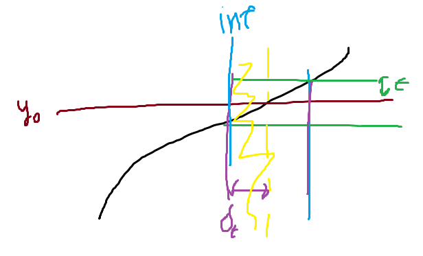
  We know that $f(i) - \epsilon > y_0$, and we know that $f(x) > f(i) - \epsilon$. Therefore, if we put this together, we have that $y_0 < f(x)$ for all $x \in(i - \delta_\epsilon, i + \delta_\epsilon)$. Therefore, these $x \in S$, and this contradicts the definition of an infimum, because $i - \delta_\epsilon < i$

  Here’s a good diagram that can help. When in doubt, always draw before you prove! The yellow scribble is the final contradiction, where we have the gap where we thought there was none.

  

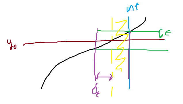
  Now, suppose that $f(i) < y_0$. Now, using the same trick, let $\epsilon = (y_0 - f(i))/2$. By definition, we know that $f(i) + \epsilon < y_0$, and $f(x) < f(i) + \epsilon$ in the span $x \in (i - \delta_\epsilon, i + \delta_\epsilon)$. Therefore, all $x \in (i, i +\delta_\epsilon) < y_0$, which means that none of $(i, i + \delta_\epsilon) \in S$, which contradicts the definition of an infimum.

  

Corollary: if $f$ is continuous on an interval $I$, then $f(I) = \{f(x) : x \in I\}$ is an interval or a single point.

• Proof

  We just need to show that given any point in a bound, it exists in $f(I)$.

  By the IVT, we know that for any $y_0, y_1 \in f(I)$, and $y_0 < y < y_1$, it is true that $y \in f(I)$.

  Pick $y_0 = \inf(f(I))$, and $y_1 = \sup(f(I))$ and some $\inf(f(I)) < y < \sup(f(I))$. If both inf and sup are in $f(I)$, then you are done. If either of them are not, then you can just select another $y_0, y_1$ such that $y_0 < y < y_1$, and you are done.

Uniform Continuity

The formal definition 🐧

A function is uniformly continuous across $S$ if for any $x, y \in S$ and any $\epsilon > 0$, there exists a $\delta_\epsilon > 0$ such that $|f(x) - f(y)| < \epsilon$ when $|x - y| < \delta_\epsilon$.

• we can always replace $x, y$ with convergent sequences as long as they converge to the same value. You can prove this by letting $\epsilon’ = \delta_\epsilon$, and you know that with large enough $n$, $|x_n - y_n| < \delta_\epsilon$.

Why do we care about uniform continuity? And what makes it different from normal continuity? Well, for normal continuity, there are cases where this $\delta_\epsilon$ depends on $\epsilon$ as well as $x_0$. Consider the example of $y - x^2$. As this $x$ becomes larger, for any $\epsilon$, we have that the $\delta_\epsilon$ becomes smaller. (we will formalize this intuition when we talk about derivatives)

As a result of our definition above, a function that is uniformly continuous has one $\delta_\epsilon$ per $\epsilon$ that works for all $x \in S$. (alternative definition)

• As a practical definition, you can also show that $\delta_\epsilon$ depends on $x_0$ but is finite in the bound.

• Examples and counterexamples

  The function $f(x) = 1/x$ is not uniformly continuous over the interval $(0, 1)$. We can create a sequence $x_n = 1/n$ and $y_n = 1/(n+1)$ such that every $x_n, y_n \in (0, 1)$. We can show that for some $n > N_\epsilon$, we have $|x_n - y_n| < \delta_\epsilon$. However, we also know that $f(x_n) = n, f(y_n) = n+1$. Therefore, $|f(x_n) - f(y_n)| = 1 > \epsilon$. This is a contradiction.

  The function $f(x) = x$ is uniformly continuous over $[0, 1]$. You can set $\delta_\epsilon = \epsilon$, and note that it doesn’t depend on $x$.

  The function $f(x) = x^2$ is uniformly continuous on $[0, 1]$. You get $|y^2 - x^2| < \epsilon$, which yields $y - x_0 \leq \sqrt{x_0^2 + \epsilon} - |x_0| = \delta_\epsilon$, which is bounded in the interval.

Continuity Theorem 🚀 ⭐

Theorem: if $f(x)$ is continuous in a closed and bounded $S$, then it is uniformly continuous. This only works on closed and bounded (compact) sets.

• Proof (contradiction)

  Suppose that $f$ is continuous but not uniformly continuous. If this is the case, then there exists some $x_n, y_n \in S$ such that $\lim |x_n - y_n| = 0$ but $|f(x_n) - f(y_n)| > \epsilon$ for some $\epsilon$ and all $x_n$. .

  ☝

  Again, just because $\lim |x_n - y_n| = 0$ doesn’t mean that $x_n, y_n$ converges. What if they oscillate in tandem?

  Now, because $S$ is closed and bounded, the BW theorem tells us that we can construct a subsequence $x_{b_k}$ such that $\lim x_{b_k} = X$. Therefore, because $f$ is continuous, we have that $\lim f(x_{b_k}) = f(\lim x_{b_k}) = f(X)$. Now, it is clear that $X = \lim y_{b_k}$ for the same sequence. Because if this were not true, then it can’t be that $\lim |x_{b_k} - y_{b_k}|$ converges to $0$.

  Therefore, we have $\lim f(x_{b_k}) = \lim f( y_{b_k})$, which means that there exists some $k > K_\epsilon$ such that $|f(x_{b_k} - f(y_{b_k})| < \epsilon$, and this is a contradiction from our original claim.

Cauchy equivalence 🚀

Theorem: if $f$ is uniformly continuous on $S$, and $s_n$ is cauchy in $S$, then $f(s_n)$ is cauchy.

• Proof (simple definitions)

  For $|x - y| < \delta$, we have $|f(x) - f(y)| < \epsilon$. By cauchy definitions, $|s_n - s_m| < \delta$ for $n, m > N_\delta$. Therefore, we have $|f(s_n) - f(s_m)| < \epsilon$ for $n, m > N_\delta$, and this is exactly the cauchy definition.

The ultimate connection 🚀 ⭐

Theorem: a real-valued function $f$ on $(a, b)$ is uniformly continuous on $(a, b)$ if and only if it can be extended to a continuous function $f$ on $[a, b]$.

We define an extension as finding $f(a), f(b)$ such that $f(x)$ is continuous at $a, b$.

• Examples and counterexamples

  We know that $1/x$ is not uniformly continuous on $(0, 1)$ because we can’t extend $1/x$ at $0$ to anything finite. Here, we see where continuity and uniform continuity is slightly different. We know that $1/x$ is continuous on $(0, 1)$ but it is not uniformly continuous.

  We know that $\sin(x)/x$ is uniformly continuous on $(0, 1)$ because it’s possible to extend $\sin(x)/x$ with $f(0) = 0$, and this gives you a continuous function.

• Proof (sequence technique + cauchy)

  The backward direction can be taken from our previous result. If $f$ can be extended to a continuous function on $[a, b]$, then we have shown that $f$ is uniformly continuous on $[a, b]$, which means that it’s uniformly continuous on $(a, b)$.

  The forward direction, we want to propose some $f(a)$ using our knowledge of uniform continuity and show that it is continuous.

  We can create a sequence $x_n \in (a, b)$ such that $\lim x_n = a$. Now, let’s define $f(a) = \lim f(x_n)$. Now, note that we can’t push in the limit because we haven’t shown that $f$ is continuous yet!

  Because $x_n$ converges, it is cauchy. From our previous proof, we know that $f(x_n)$ is cauchy. Therefore, we know that it converges. This is good, but the problem is that we don’t know if the limit is well-defined. It could be that the limit depends on your choice of $x_n$.

  ☝

  Why? Well, consider $\sin(1/x)$. Depending on how you approach $0$ with $x_n$, you can get completely different results!

  So now, we select another $\tilde x_n$. Similarly, we know that $\lim f(\tilde x_n)$ converges. We can create a larger sequence $X_n$ such that $X_{2n} = \tilde x_n$ and $X_{2n + 1} = x_n$. By construction, it is obvious that $\lim X = a$. We know that $\lim f(X_n)$ exists, and because $f(x_n)$ and $f(\tilde x_n)$ are subsequences of $f(X_n)$, we conclude that $\lim f(x_n) = \lim f(\tilde x_n)$.

  If we set $f(a)$ to this value, we have shown that $f(\lim_{x \rightarrow a} x) = \lim_{x \rightarrow a} f(x)$. A similar thing can be done for $b$, which means that $f$ can be extended to be continuous on $[a, b]$.

Real Roots Development 🧸

This is just a fun aside, but how do we define $a^x$ for $x \in \mathbb{R}$? We start from the natural numbers

1. We define $a^x, x \in N$ to be $a * a * a …$ for $x$ times.

2. We define $a^x, x \in Q$ to be the following. Suppose we have $x = m / n$. Then, $a^x$ is a number such that $(a^x)^n = a^m$.

3. Now, we define $a^x, x \in R$ to be the following: create a sequence $\{q_i\} \in Q$ such that $\lim q_i = x$. (this is almost like a dedekind cut). We define $a^x = \lim a^{q_i}$.

This last part suffers from the same non-determinism that our last section dealt with. It is possible to show that all such $q_i$ converges to the same value of $a^x$, but we won’t get into that here.