Multivariate Gaussians

We write the output as $X \sim \mathcal{N}(\mu, \Sigma)$, and $X$ is a random vector.

The covariance matrix determines its shape. It's not exactly the quadratic form specified by the covariance matrix, as much as you are tempted to do so. Rather, you can think of the off-diagonals as a sort of "correlation". As such, if the matrix was like

You can imagine that the distribution is tilted such that the major axis is in line with $y = x$ (or roughly so), because we have a positive correlation between the two random variables.

Relationship to Univariate

Recall that the univariate is

You can imagine extending the idea of a quadratic inside the exponent to that of a quadratic form. Now, because $\Sigma$ is positive definite, we also know that $\Sigma^{-1}$ is positive definite. As such, we know that the whole expression $-1/2 (x - \mu)^T \Sigma^{-1} (x - \mu) < 0$, which is very helpful.

Just like the univariate, the multinormal has a constant out front such that

Covariance matrix

Recall that covariance is defined as

The covariance matrix is defined as $\Sigma_{ij} = Cov(X_i, X_j)$. Because the covariance operation is symmetric, $\Sigma$ is also symmetric.

Identity: relating covariance matrix to expectation

As an identity, note that

The proof:

We know that $\Sigma = E[(X - \mu)(X - \mu)^T]$ just by the definition of covariance.

• $E[(X - \mu)(X - \mu)^T] = E[XX^T - X\mu^T - \mu X^T + \mu \mu^T]$

• $= E[XX^T] - \mu \mu^T - \mu \mu^T + \mu \mu^T$

• $= E[XX^T] - \mu \mu^T$

Proposition: $\Sigma$ is positive definite

The proof starts with $z^T \Sigma z$. You write it out as a sum, and then you add in the official definition of covariance.

Now, this form with the double summation and the $i, j$ terms repeating should ring a bell. You can recast this as

Of course, this means that the thing inside the expectation is always non-negative. Expectation of a non-negative number returns a non-negative number, completing one part of our proof. We know that $\Sigma$ is positive semidefinite. We can actually make it stronger and say that it's positive definite, because it must always be invertible.

Diagonal Covariance

A multivariate gaussian with a diagonal covariance just means that it's the product of $n$ independent gaussian distributions. This means that there is no "dependence" between the gaussians on each dimension. Visually, it means that the major axes of the gaussian lie on the coordinate axes.

Isocontours

Is it possible to see the contours of the gaussian? Yes!

Diagonal isocontours

In the 2d case, the isocontours of a diagonal multivariate distribution is just an ellipse

Intuitively, a non-diagonal multivariate distribution is just a rotated ellipse, though that formula becomes very complicated.

In higher dimensions, these isocontours are just ellipsoids.

The smaller the variance, the shorter the axis length of the ellipsoid is in that direction.

Linear transformation interpretation (important)

Theorem: every multivariate gaussian is a linear mapping from $\mathcal{N}(0, I)$.

This actually makes a lot of sense. $\mathcal{N}(0, 1)$ is composed of independent gaussians, and we can stretch/shrink the distribtion using a scaling factor and shift it with a constant offset. The scaling factor is a matrix, which can intertwine the independent gaussians to produce a non-diagonal covariance output.

• Proof

  This is not trivial, but it does some neat work on the $\Sigma$. First, we know that $\Sigma$ can be factorized into $U D U^T$ because it's symmetric, where $U$ is an orthogonal eigenbasis.

  We can introduce the notion of a square root:

  

  Which means that we can rewrite this as

  

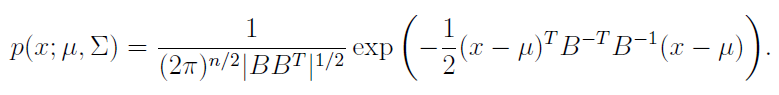
  Now we can apply the change of variable formula (see probability section) to get

  

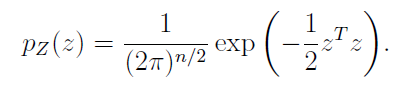
  (don't worry too much about this at the moment). All you need to see is that with some linear transformation (change of variable) we were able to get our $p(x)$ into a generic gaussian

Gaussian Integrals

Gaussian integrals have closed form solutions. The first one is just the distribution definition, the second one is the expectation, and the third one is the variance

Multivariate gaussians and block matrices

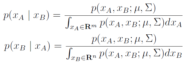
Suppose we had a vector-valued random variable that is consisted of two different vectors

We'd have a mean and a covariance matrix based on this $x$. The covariance matrix is a block matrix

if $x_1$ was length $r$ and $x_2$ was length $s$, then $\Sigma_{11}$ would be $r\times r$, $\Sigma_{12}$ would be $r\times s$, and so on. We also know that by symmetry, $\Sigma_{21} = \Sigma_{12}^T$.

When dealing with block matrices, we have that

And here's the magic of block matrices! These are almost like numbers and you can treat them as such.

The marginal distribution of $x_1$ is just $\mathcal{N}(\mu_1, \Sigma_{11})$ and the same pattern for $x_2$. You can show that the conditional distribution is just

Below, we will explore some of these properties in greater detail.

Closure properties

Gaussians are closed under three operations

• sum

• marginal

• conditional

Sum

The mean is obvious, because of the linearity of expectation.

The covariance matrix is derived with a bit more algebraic hardship

and we use independence $E[z_i y_j] = E[z_i]E[y_j]$ to get our final form

We will not show here why the sum is actually a gaussian. This is just a lot of algebraic hardship with the convolution operator. But we have proved that the covariance matrix and the mean vector do obey certain rules

Marginal

If you had two random vectors $x_A, x_B$ distributed as

then the marginals are gaussian: (yes, we use a block matrix setup here)

The proof is pretty involved, but it's also more algebraic hardship including a whole complete-the-squares thing with matrices. The integral disappears because we eventually see an integral across a proper distribution, which is just $1$

Conditional

Now this one is probably the most interesting. If we had the same setup as above and instead took the conditional expression, we would have

and we claim that

The proof is also pretty involved, and it does the same completing the squares trick. We will be using this closure property in gaussian process