Exponential Family Distributions

Recall that when we learned about MRF, our probability distribution was

where $f$ was just a concatenation of indicator variables and $\theta_c$ was the log factors for each configuration.

We can generalize this!

Definitions

We define an exponential family as

where

• $h$ is the base measure (often a constant)

• $w$ are the natural parameters

• $f(x)$ are the sufficient statistics

• and $A(w)$ is the log-partition function, defined as

Making exponential families

Start with taking $\exp \log$ of the expression, which reduces it down into a form that is most similar to the exponential family. Take a look at the coefficient behind $x$. This is your $w$. You might get a $A(\theta)$, where $\theta$ is the parameter of your original distribtuion. Your goal is to get $A(w)$, so derive $\theta = f(w)$ and plug that in.

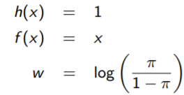
Example: bernoulli

Here, we see the formula condense down

(note that the second step of reduction isn’t necessary; you can just consolidate like terms after you take the log.)

You immediately get the following things

and after solving for $\pi$ in terms of $w$, you get

Example: Gaussian

The key for a gaussian is to push the $\sigma$ inside the exponent because it is a parameter of the distribution

Therefore, we can define

We can solve for $\sigma$ and $\mu$ in terms of the natural parameters, which gets us

Sufficient Statistic

The sufficient statistic actually has a meaning. It fully “summarizes” the data. This is because if you had multiple data points in $D$, a dataset, and you wanted to compute the MLE of $w$, you get

and you see that the likelihood for $w$ depends only on $f(x_m)$. A similar result can be said for the posterior $p(w| D)$ s

Statistics, generalized

We define a statistic of some random sample $X_1, ... X_m$ as $T(X_1, ..., X_m)$. We might recognize the classics, like max, median, mode, mean ,etc.

We define a statistic as sufficient for parameter $w$ if the conditional distribution of $w$ given some statistic $T$ is totally independent of $X_1, ..., X_m$. More intuitively, this statistic “boils down” all the important information for us.

Formally, we say that

Sufficient statistics are hard to come by, the they are easy for exponential families.

Proving that $f$ is sufficient

We want to show that $x \perp w | f(x)$. Our approach: find $p(x | f = f, w)$ and show that the expression doesn’t depend on $w$.

essentially, if $x, f$ match, we have the normal probability. Else, we havec $0$. We realize that the final expression has one $w$ term (the $\exp$), but it cancels out.

Derivatives and convexity

Let’s look at some nice properties of the exponential distribution.

Derivative of log normalizer

If you take the derivative of the log normalizer, you can push the derivative into the integral to get

the second step is derived from how the denominator is just the exponential of $A$. So the key upshot is that derivative is the moment of the sufficient satistic. In other words, it is the “average” value based on the distribution parameterized by $w$

Convexity of log normalizer

You can show (DO THIS AS AN EXERCISE) that the hessian of the log normalizer is just the covariance of $f(x)$

which means that $A(w)$ is a convex function of $w$ (it means that it has a minimum). When we subtract this from the exponential distribution, we are essentially adding a linear function to a concave function, which makes the log-probability concave.

What does this mean?

To sum things up, the $w^Tf$ term is linear, and the $A(w)$ term is convex. Therefore, the negative log likelihood is convex.

Minimal representations

Ideally, we want a sufficient statistic that is linearly independent. In other words, there is no $a\cdot f(x) = c$ where $a$ is non-zero. When this happens, we call it minimal.

If this condition is not satisfied, we call the exponential family as overcomplete. Because this would mean that $w^Tf(x) \propto (w + a)^Tf(x)$, or in other words,

We want a unique $w$ associated with each distribution, but when it’s overcomplete, this is not the case. A good example is the two forms of Bernoulli representation you might come up with

The first one has two values in $f(x)$, but the vector $[1, 1]\cdot f(x) = 1$ for all $x$, which implies that it is overcomplete.

Mapping between moments and distributions

Here, we want to show something very neat about moments and distributions.

The moment of a distribution is the expectation of something. In the case of the exponential family, we derived that the gradient of the log-partition function is the moment of the statistic

If the exponential family is minimal, we can solve for $w$ from the moment. This is actually a very roudnabout way of saying something that should be relatively obvious. The parameters of the distribution are typically related to some sort of mean.

• example from gaussian

  

  

  and the derivative WRT $w_2$ yields $E[x^2]$. From these two, we can solve for $\mu, \sigma$.

This observation can be generalized. We will actually show that one way is inference, and the other way is learning.

Moments as inference

Remember that the moment is just the gradient of the log partition function. However, to compute this, we need to do an inference problem!

For example, let’s look at the gradient in the case of an MRF. To compute the expectation, we need to look at each individual component, which corresponds to a marginalization. For example, we can just let $f(x)$ be a selection function, as shown below, to get our marginalization.

Reverse moments as learning

Suppose that we had $Q$ as an exponential family and $p(x)$ as some distribution. To fit $Q$ to $p$, we have the following objective

We call this the moment projection or the M-projection. It can be shown that if you can find some $w^*$ such that $E_{q(x ; w^*)}[f(x)] = E_p[f(x)]$, then the M-projection of $p$ onto $Q$ is just $q(x; w^*)$.

We can prove this through the following idea. Let’s calculate $D(p||q_w)$ and $D(p || q_{w^*})$ and how that the latter is always smaller, so it has got to be the M-projection. We do this by doing some algebraic hardship

Note that the summation applies to all of the thing after the summation, not just the $p(x)f(x)$.

Now, we realize that the summation is just $E_{p}[f(x)]$. When we moment-matched, we set

So we can replace that summation with the equivalent expectation. Note that we use this abuse of notation with the $|$ symbolizing parameterization.

We arrive at the last equation when we add a $\log \exp$. Essentially, we rebuild the same expression as line $1$, but instead of $p(x)$, we have $q(x;w^*)$. This all relied on the knowledge of moment matching.

This shows that the minimum distance of distributions is a M-matching.

Zooming out

So we saw that deriving the optimal parameters is an optimization problem, and what’s more, it can be done by matching moments. So we have the reverse, from moments to parameters.

Again, recall that the forward mapping is from parameters to moments, which are done through inference-type operations. You take the expectation across the log partition function, which requires you to sample from $p(x | w)$, which depends on the $w$.

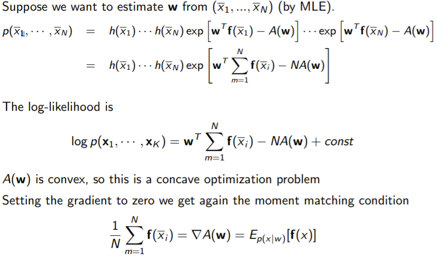
Learning and maximum likelihood

if we have $p(x | w)$ is in the exponential family, then DKL between empirical $\hat p$ and $p(x | w)$ is minimized when

(take a second to think about this). The key upshot is that the MLE is doing moment matching!

You can also show that by manually optimizing the log likelihood, you get the same thing

• Derivation

  

Maximum Entropy

We can also show that exponential family distributions maximize the entropy $H(p)$ over all distributions whose moments match

For example, the gaussian is the most entropic distribution whose mean is $\mu$ and whose variance is $\sigma$. The big idea is that we make everything as chaotic as possible, given that it satisfies the moments we desire.

We can show this by optimizing the entropy subject to the moment