What are we trying to do?

We are trying to optimize the same thing

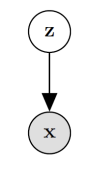
The curse of the E step

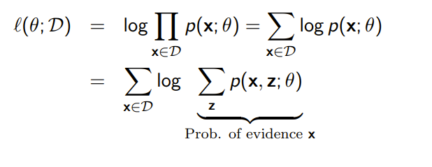
Remember what we were worried about in the E step when we first stalked about the EM algorithm? We saw that we needed to compute

The joint distribution is assumed to be easy, but the marginal $p(x)$ was only tractable because $z$ was a scalar random variable that took only a few values. What if $z$ were something arbitrary, like another random vector?

Reframing EM learning

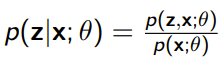
If we use the variational mindset and start trying to approximate $p(z|x)$, we get the following:

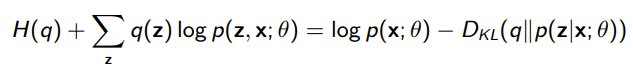
and this yields

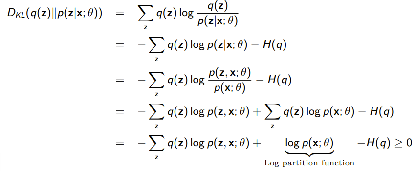
so in our discussion on variational inference, we hinted at why we might find the log partition function to be useful. In an MRF, it helps us compute a conditional distribution. Here, it helps us compute the overall objective.

This is what we were talking about when we said that the log partition function had special meaning sometimes!

Here, we have shown through a variational lens, the same EM lower bound!

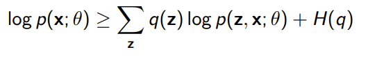
ELBO objective

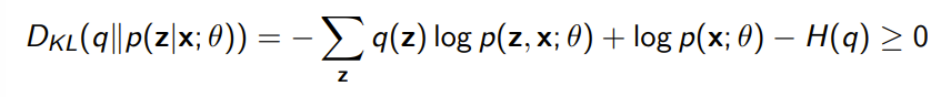
From our variational derivation, however, we can also derive the following equality:

and we assign function $F[q, \theta]$ equal to the two values. You can understand the equality above as two different ideologies that yield the same answer.

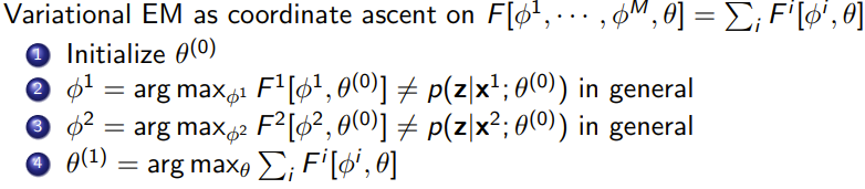
We can understand the EM algorithm as performing coordinate ascent on $F$.

1. Start with $F[q_0, \theta_0]$

2. Optimize $q$ using the right hand side of the equality. The only term that matters is the KL divergence

3. Optimize $\theta$ using the left hand side of the equality. Note how the only component that matters is the $\sum_z q(z)\log p(z, x)$

At every step, if we assume that we can let $q(z) = p(z | x)$, we have $\log p(x, \theta_0) = F[q_0, \theta_0] \leq F[q_0, \theta_1]$. And then we have $\log p(x, \theta_1) = F[q_1, \theta_1]$ and so on. As if we haven’t had enough analogies already, you can think of a person pushing a box up a steep incline. First, they will push it as far up as they can with their arms (M step), and then they will walk up the incline until they are level with the box (E step), and then they repeat.

Because you are doing coordinate ascent, the objective, which is related to the $F$, never decreases.

Variational EM

Previously, we used a variational framework to derive another EM expression, but then we assumed that we could find $q = p(z | x)$ tractably. Now, we will remove this assumption.

The derivation

Now, consider the case where $p(z | x)$ is not tractable. If you use some approximation $q$, this still holds

from this expression and the inequality to $0$, you get that

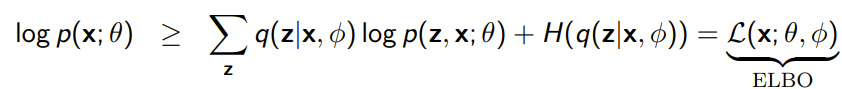
. Note that we use $\phi$ to parameterize this $q$, which means that the ELBO objective is optimized by alternating optimization over $\theta, \phi$. We understand here that the likelihood is still lower bounded by the ELBO objective, no matter what $q$ we use.

However, from the equality expression, you also get that

which means that there is some distance between the likelihood and the ELBO objective. Graphically, this looks like this

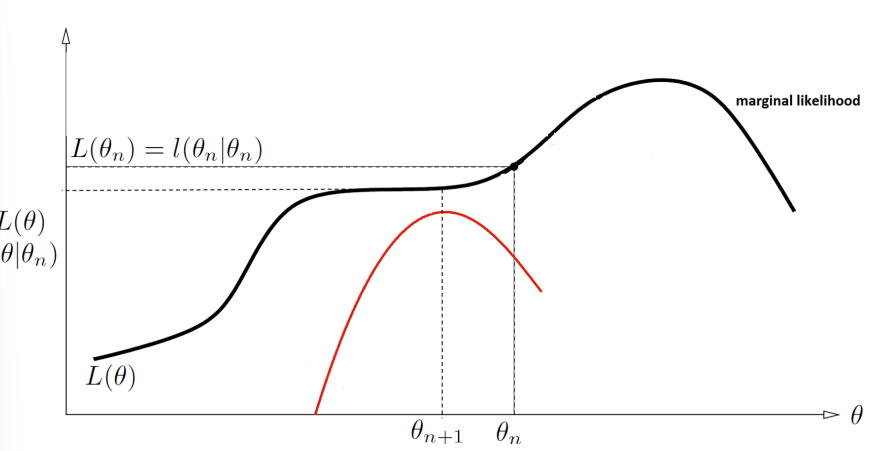
The algorithm

We need a $\phi^i$ for each data point, which parameterizes $q(z; \phi^i) \approx p(z| x^i)$. In the E step, you optimize each $\phi$ to minimize the KL divergence between $q(z; \phi^i)$ and $p(z | x^i)$.

Computing the variational objective

Here, we arrive at the big question. We’ve set things up in terms of variational inference, but how exactly do we compute $\arg \max_\phi$? We’ve seen previous techniques on exponential families, which included the mean field and the relaxation. These are totally valid, but can we generalize to an arbitrary function?

It turns out that, yes, we can! It takes a little bit of mathematical gymnastics though. We can understand a function $q$ as being parameterized by $\phi^i$, such that $q(z; \phi^i)\approx p(z | x^i)$. How, we can define a function $f$ of functions that map $x^i \rightarrow \phi^i$. In other words, this function $f$ will generate a function that best approximates a certain posterior distribution!

Why does this help? Well, as we recall, the big trouble with variational inference is the optimization in the function space. We used things like Moments and stuff, just so we could move away from functions. But if we can parameterize functions, and if we can parameterize $f$ through $\phi$, then we can just do gradeint ascent!

Indeed, for more expressive models, this is exactly what we do. To talk about how we might do this, let’s look at a specific example below.

Deep generative models and the variational objective

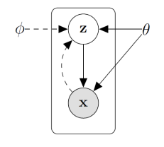
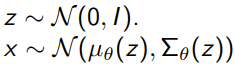
Here, we will solve this problem by looking at a specific case of the the deep generative model. These models look like this:

and we have $p(x | z; \theta)$ and $p(z; \theta)$. So $\theta$ is the generative parameter. We also have $q_\phi(z | x)$, shown in the dotted line. This is the $f$ we were talking about in the previous section! With this function of functions (implicit), we are able to estimate the posterior.

Note how the forward and backward relationships are parameterized by different things. Normally, this is not needed but we do this because the inversion of the arrow is intractable

Optimizing Lower Bound

And if we write out the objective, we get

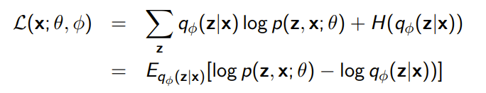
To optimize this, we just need to perform joint gradient ascent on $\theta$ and $\phi$

Optimizing $\theta$

This is the M step, and it is quite simple. We just use a monte carlo estimate of the expectation, and we push the gradient inside

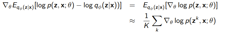
This is no different than any other EM algorithm

Optimizing $\phi$

Now this is the variational part! Our initial idea is that we can just take the gradient as usual. However, we note that the expectation contains the parameter, and this isn’t good. We would like to use a Monte Carlo approximation of the expectation, but we can’t do it if the sampling process itself is being optimized.

Instead, we turn to a little technique called REINFORCE, which is used in reinforcement learning.

Let’s say we have a simple objective $E_{q_\phi(z)}[r(z)]$ and we wanted to take the gradient. We use a cool math trick that we used a lot in this course, which is to multiply by $1$ in an intelligent manner

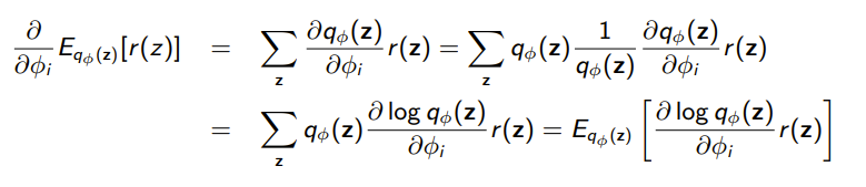
The key insight is that we want to turn the gradient of an expectation into an expectation itself, and we do this in an importance sampling-esque way. The $\log$ is just an insight of how derivative of logarithms work.

From this, we can construct a monte carlo estimate of $\nabla_\phi$ as follows:

The second term in the expectation is because in the case of our EM algorithm, the expectation value also depends on $\phi$, which leads to some more mathematical complexity that we won’t get too much into. But essentially this yields the additional term that wasn’t present in the REINFORCE bare example.

The reparameterization trick!

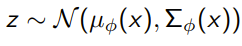
Unfortunately, as the RL domain knows quite well, this policy gradient trick is very high variance and needs a lot of data. We can also use a reparameterization trick if the $q$ is a gaussian. Essentially, we sample from $\mathcal{N}(0, 1)$ and then transform it into $q_\phi$ through a linear transformation of the sample. This works because of certain properties of the gaussian, but it doesn’t work in the general case. This is where the REINFORCE thing can help, but there’s no free lunch.

The crux of the problem is that we're taking the expectation through $Q$, which depends on $\psi, \phi$. What if we "moved" the randomness like this:

such that $\epsilon \sim \mathcal{N}(0, I)$? Instead of having one distribution $Q_i$, we've resorted to transforming a vanilla multivariate gaussian

In this manner, we can rewrite the ELBO objective as

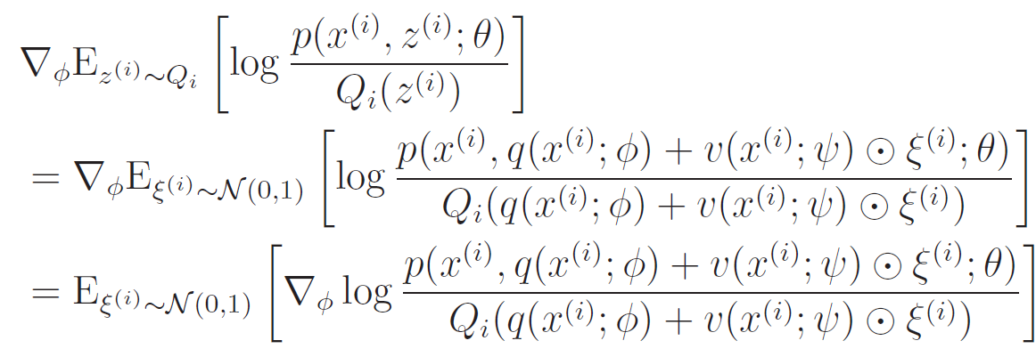
And this is easy to propagate a gradient through. The gradient of an expectation is just the expectation of the gradient, and we often just sample from the dataset to form the "expectation"

Variational Autoencoder

We just use what we derived before, but we specify neural networks for $p(x | z)$ and $q(z | x)$. More specifically, we might have the generative model be

(the neural networks are for the mu and the sigma)

and you might have the variational inference model be

and so you will have a structure like

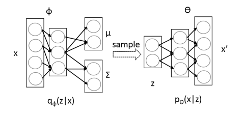
During runtime, you ditch the $q$ and you sample $z$ uniformly. The $q$ is for training purposes, as we have seen through the EM formulation