The two types of questions

1. Marginal inference: given a joint distribution, what is the marginal probability of one variable?

2. Maximum a posteriori: given evidence, what is the most likely assignment to the other variables in the model?

Much of the time, these problems are actually NP hard. However, we can use approximate inference, and some special graph structures have nice solutions.

Our first inference algorithm is variable elimination. This is an exact form of inference, meaning that there is no approximation involved.

The setup

In both cases, we want to find some conditional $p(Y | E = e)$, which means that you want to calculate

Your joint distribution has variable sets $Y, E$, and $W$. This $W$ is the unobserved variables that you have to marginalize out, as follows:

Now, for marginal probability inference, that expression above is enough. For MAP inference, you just want to find

And for marginal MAP, you just want to find

The problem

These things seem pretty simple, but there’s an important catch: as the set $W$ becomes large, the number of summations in $\sum_w$ becomes exponentially large. This, of course, becomes intractable.

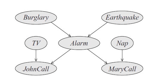
In fact, inference on a graph is an NP hard problem. We can show this pretty easily. We consider the SAT problem, which is an NP complete problem. In this problem, we want to see if something like

has a solution. If we let each node in the graph be a boolean variable, and let each factor in the graph be one of the triplet clauses, we can model SAT. More specfically, let each of the factors return 1 if it’s satisfied and 0 if it’s not. The product of factors is the joint distribution, but it’s also the answer to the boolean expression.

Therefore, to find $\arg \max_{x_1, .. x_n}p(X_1, ..., X_n)$ is to solve SAT, which we know is NP complete. Similarly, the normalization constant in this expression is also hard to compute.

What does this mean?

It means that there exists certain graphs such that inference is NP hard. However, other graphs are very easy to do inference in, like hidden markov models and other tree-structured graphs.

However, in general terms, it means that we often have to work smarter when it comes to inference. Enter dynamic programming.

Distributive law

When dealing with sum-product formulation, we can “push” the summation into the product. This takes a hot second to understand, so we can first understand the special case

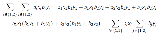
You see how we can regroup by like terms because the inner summation doesn’t care about $a_ix_i$? We can generalize this to the following:

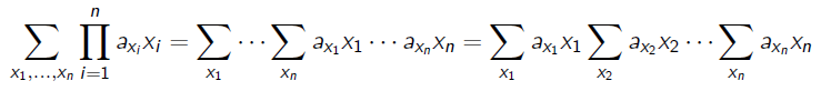
Dynamic programming approach

Suppose we wanted to find a marginal probability. We can write it as

This is a correct naive approach, but we aren’t using our factorizations! Why don’t we split up the summations?

Now, we compute the sums from inside to out. Each sum will remove one variable and depend on another, until the last one which ends the chain. We actually call this dynamic programming because perform a sequence of smaller problems, and this contributes to the final answer. This is an exponential decrease in time. Previously it was $k^n$, and now it’s $O(nk^2)$.

Formally, we cache and reuse computation, which allows us to do inference over the joint without ever calculating it!

Sum Product inference: generalizing

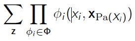
Let’s represent our distribution as a product of factors, where $\phi(x_1, PA(X_i)) = p(x_i | x_{Pa(X_i)})$. The joint probability looks like

Just to unpack this real quick: we assign each variable a factor that is the CPD of that variable.

When we marginalize over variables $Z$, we want to compute

We define $scope(\phi_i) = \{x_i, Pa(x_i)\}$. This is useful in our later discussion.

Factor marginalization

Before we go on, let’s understand what factor marginalization means. In other words, what does this mean?

In essence, you are making a new factor $\phi(a)$ that depends only on $a$. Tabularly, it looks like this:

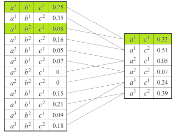
Geometrically, it’s like summing along one dimension, if you think of a factor as a multidimensional table.

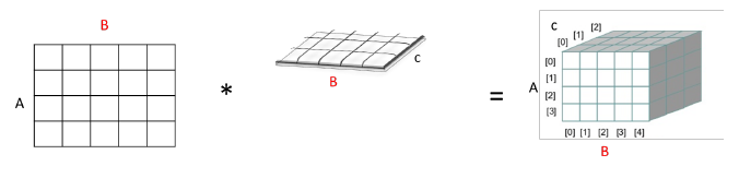
Factor combination

What about this?

Well, from this you can always make a new factor $\phi(a, b, c)$ that covers all the dependencies in the product above. However, do beware that you are making a new edge in the dependency graph. However, this is often needed for factor marginalization because you need to group all factors with some variable inside of it.

Geometrically, it’s just expanding the dimensions of one table

Variable Elimination: the algorithm

Let $Z$ be the set that you want to eliminate. First, order the set $Z$ as $Z_1,..., Z_k$. This is known as the elimination ordering. Now, for each $Z_i$ in $Z$:

1. Multiply all factors in the graph that have $Z_i$ within their scope. This means that it is either referring to $Z_i$ of is a child of $Z_i$. This should make a new factor. These intermediate factors are not necessairly valid probability distributions.

2. Marginalize the product over $Z_i$. This generates a smaller factor, and add this smaller factor back in. We typically denote the smaller factor as $\tau$.

3. Remove the original factors that contributed to step 1.

The problem of ordering

If you get a perfect ordering, each step will multiply two factors together to form a two-variable factor (think about the markov assumption). Then, when you marginalize, you end up with a one-variable factor. Using this, you can make the next two-variable factor. The key part of this is that you don’t accumulate unmarginalized factors.

However, if you’re unlucky, you will actually accumulate unmarginalized factors such that at the end of the day, the computation may end up tending to be exponential.

Knowing the right order is an NP hard problem!

Introducing evidence

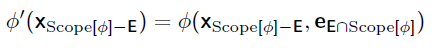
Say you want to calculate $p(Y | E = e)$. You need $P(Y, e)$ and $P(e)$. Note the difference in capital vs lower case. You want to introduce evidence into the graph. To do this, you need to apply variable elimination to the joint distribution $p(Y, E, W)$. When you have $p(Y, E)$, just plug in the evidence. We define this rigorously as

This gets you $P(Y | E = e)$. Graphically, it looks like slicing a factor

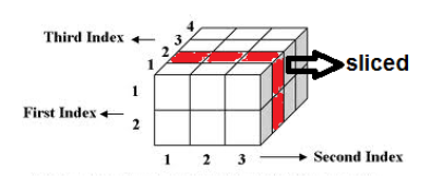
After that, you sum over $Y$ to get $p(e)$, and then you are done!

Adapting to MRF

This is trivial. Previously we define $\phi$ specifically in terms of the CPD. Now, you just use the existing $\phi$.

Runtime complexity

In the best case, it’s polynomial in $k$ because things tend to collapse as you move your way down. However, this may not always be the case. If you did it the wrong way, you might be pinned against a wall and start building up larger and larger factors without ever removing anything until the very end, which means that you gain no improvement over a naive summation.

More rigorously, it’s $O(nk^{N_{MAX}})$ where $N_{MAX}$ is the maximum number of variables in the accumulated factor. In the best case $N_{MAX} = 2$, but it can be as large as $n$.

Nuances on runtime complexity

When you think elimination complexity, think “how large is the joint factor table once I remove a variable?” For example, if the graph were $A -B-C$, when I remove $A$, the table I need to sum across just has $k^2$ values because it contains $A, B$ which both have $k$ possible values.

The key thing is once I remove a variable, not what comes before. Because when you remove a variable, you create more connections.

Graph interpretation of runtime

When we turn a bayes net into the form we need for variable elimination, we moralize the network. We didn’t talk about this much above, but you can understand why this happens when we smush the different factors together. Here’s what the two steps of elimination look like on the graph

1. When we concatenate all factors together, we create a clique involving all these factors. These new edges created are called fill edges

2. When we remove the variable (marginalize it out), we just remove the variable and its incident connections

The computation cost can be represented as a single graph, where we union all the fill edges created during computation. We call this the induced graph $I_{\Phi, \prec}$ where $\prec$ (\prec) is the elimination ordering.

• Great example

  

Now, here’s the interesting theory

• every factor that is generated during VE has a scope that is a clique in $I$. Intuitively this is true because when we remove that factor, we must create a clique

• Every maximal clique is the scope of some intermediate factor. This is the converse of the above statement, and intuitively it should also make sense

⇒ Upshot: $N_{max}$ is equal to the largest clique in $I_{\phi, \prec}$.

⇒ Upshot of the upshot: when you start removing nodes from a graph, it’s a bad move to remove a node that is highly connected because you need to interconnect everything! And the more connections, the more connections you need to make later. You accumulate complexity.

Treewidth

We define the width of an induced graph is the number of nodes in the largest clique minus one. We then define the induced width as the width of the graph induced by applying variable elimination with ordering $\prec$.

We define the treewidth of a graph $G$ as

The key point here is that the treewidth is the largest clique you get when you apply the best possible elimination ordering.

It’s kinda like “how close to a tree is this graph?” If you plug in a tree, the largest clique you induce minimally is just $2$, so the treewidth is 1.

Optimizing the order

Again, we can’t really pick the right order by inspection as it is NP-hard. However, we have a few strategies

1. pick the variable that has the fewest neighbors. This is a greedy approach (min-neighbor)

2. pick the variables that minimize the cardinalities of the dependent variables (min-weight)

3. Choose vertices that minimizes the size of the factor that will be added (min fill)

Often these three strategies will agree on which variable you want to eliminate.

Removing variables in directed models

This one is very interesting. Given a graph, how do you remove a variable from the graph without adding additional independencies that weren’t there before? We did this with MRF’s, but can we do it directly with Bayesian networks?

There’s a simple algorithm for removing node $x_i$.

1. make the children of $x_i$ densely connected in some arbitrary order

2. connect the parents of $x_i$ pairwise to the children of $x_i$

3. Keeping the arbitrary order, connect the parents of the children of $x_i$ to the children of $x_i$ that come after this current child in the arbitrary order.

The first step is because $x_i$ makes any pairwise children have active paths, so we need to keep this. The second step keeps the cascades from parents to children. The third step keeps the v-structures from parents of children to other children. We use the convoluted assigning order in order to keep things minimally connected. We don’t connect to children before the current child in step 3 because the dense connection in step 1 creates a v-structure already. This takes a lot of thinking!