Motivation

The problem here is that often our models are too complex to yield us a precise answer. When treewidth is less than 25, it’s typically feasible to use exact inference. However, many real-world problems have high treewidth. When this happens, we turn to approximate solutions.

Variational methods make inference an optimization problem (variational lower bound) in which you try to estimate a multimodal distribution using a series of simpler distributions.

On the other side of things, we have sampling methods generate a distribution at random and approximate the distribution that way.

In many cases, approximations are sufficient

Monte Carlo Estimation

The big idea is that you want to express the quantity of interest as an expected value of a random variable.

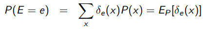
To get a marginal probability, just use an indicator function

Essentially, you’re selecting the distributions that fit what you want. Therefore, you can express it as an expectation

A monte carlo method is then used to estimate the expectation by assuming that the samples match the true probability distribution

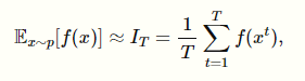
Just generate $T$ samples and take the average! And that works! By sampling, we have an unbiased estimator for the true expected value.

Properties of Monte Carlo

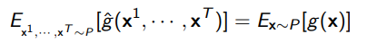
The monte carlo estimation is itself a random variable. However, it is possible to show that the expected value of the estimation is the true value

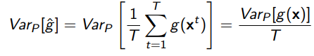
And that the variance of the monte carlo sample reaches zero as $T → \infty$ (sample size)

We can also talk about the probability that we are off by some value. The Hoeffding bound states that

and the Chernoff bound states that

Or, in other words, the error decreases exponentially.

Rejection sampling

Our big goal is to find $P(E = e)$, where $E$ is a set of variables and $Z$ is the other set of variables. Essentially, we want to find the marginal.

Rejection sampling is basically this: you sample values of $E, Z$ from a uniform distribution. Then, you select the samples that have your desired $E = e$ and then take the ratio of these samples to the total samples drawn.

Let’s write out the algorithm

1. Sample $n$ times from the joint distribution

2. Count the number of times, $k$, that $e$ shows up.

3. $P(E = e) \approx k/n$

More formally, we have

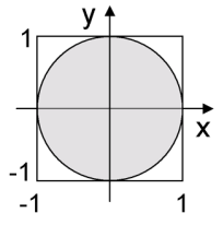
And more intuitively, we are just taking the ratio of areas. The square is your uniform distribution, and the circle is the samples that satisfy $E = e$.

Importance sampling

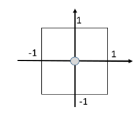
Rejection sampling is quite wasteful. Let’s say we had a very small circle. The problem is that all the information you need is inside that circle, and all other samples are useless.

This can definitely happen, because it might be the case that $P(E = e)$ is a very small chance, and yet you still want to do meaningful inference on it, like finding $P(Z = z | E = e)$.

Intuitively, we just want to have a better sampling scheme! In fact, why don’t we start by sampling inside the small circle? In other words, let’s fix the $E$ and sample only from $Z$. This would require sampling from the distribution $P(Z | E = e)$.

How can we get $P(E = e)$ from this? Well...we can use some mathematical trickery

So a monte carlo approach would be to sample from $z$ and then compute the ratio. This yields one sample perfect accuracy because $p(z, e) / p(z | e) = p(e)$, and that’s the value we’re after! There’s no need to compute more samples.

However, this is not really playing it fair, because to know $p(z | e)$ and to sample from it, we essentially need to calculate $p(z, e) / p(e)$, which yields a chicken and egg problem.

But this seems promising. Can we use a proposal distribution $Q(Z)$ that we efficiently sample from? We can still use the trick above and this gets us

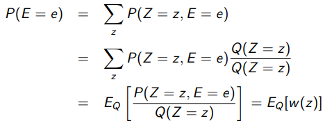
⇒ Key upshot: pick a proposal distribution, sample from that distribution and reweigh the samples to calculate the desired expectation. Now, it’s worth noting that this $Q$ must have non-zero probabilities whenever the original $P$ has non-zero probabilities, or else we might end up with a divide-by-zero

Importance sampling: intuition

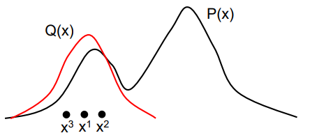
Your goal is to sample from some $p(z | e)$. If you could do this, then your problem is solved. However, you can’t do this. Therefore, you sample from a surrogate distribution and then reweigh the sample values to perform your calculations. This kinda looks like this

Importance sampling: some more intuition on chicken-egg problem

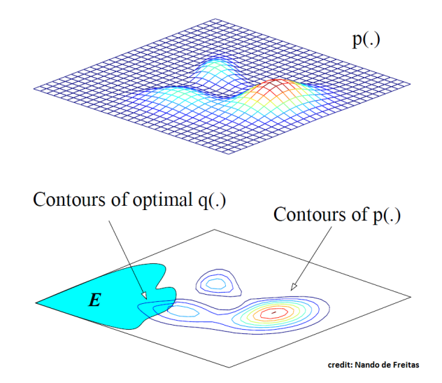
You want to find $P(E = e)$, which is the blue blob. In the best case scenario, your $q$ will be sampling the $z$ from that same region. However, to do this, we need to find the area of $E$ to normalize the distribution, and that is equivalent to finding $P(E = e)$ directly.

Therefore, we can’t sample efficiently from $P(Z | E = e)$, but what we can do is define a surrogate distribution (typically a uniform or a gaussian) that is defined for all points of $E$. You just have to reweigh the distribution probability based on $p$.

Likelihood weighting

We can use a uniform distribution or a gaussian, but can we do better? What if we defined it as

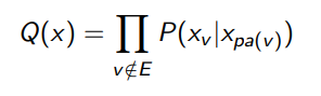
In plain english, we go back into the network and then “clamp” the evidence in each CPD table. This means that anything downstream of the observed evidence will now be sampled according to this observed evidence in mind. In other words

1. start from a topological sort

2. Sample as usual, but if you get to a variable with a CPD that has an observed variable, use this variable directly in your sampling (and not what you got before)

This is different than sampling from the original distribution $p(z | e)$ because in that case, we must do inference on the upstream variables too. What we are doing is “in between” the prior and posterior distribution. But it’s close enough!

And in fact, it has a very nice mathematical result: the weights across the expectation are very easy to calculate

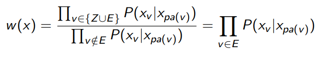
Intuitively, you’re finding an approximate version of $p(e, z) / p(z | e)$ which yields an approximation of $p(e)$, which is given by looking at the evidence nodes and computing the chance that it happened by only looking at the parents. Again, this is an approximation because the real $p(e)$ is a marginalization.

Application to RL

In RL, we have something called a policy gradient. Normally, we have to sample from the distribution of transitions that are ON policy. However, this is horribly sample inefficient. To mitigate this, we use importance sampling and let $q$ be all the past transitions

Normalized Importance Sampling

Here’s the problem. We can use monte carlo to find out approximations for $P(E = e)$, $P(E = e, X = x)$. However, we CAN’T take their quotient to find $P(X = x | E = e)$. Why? Well, we have no guarantees on which way the errors go. The errors could compound when you take the quotient, and this is not good! You can try to prove that this is no longer an unbiased estimator.

As a primitive solution, we can use the same set of samples for importance sampling

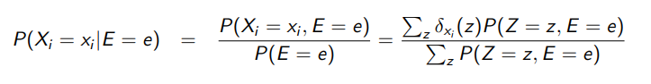
where $z$ is all the variables that are not $e$, and $\delta_{x_i}(z)$ is 1 if $z$ contains the valid $x_i$, and 0 if not.

To estimate the numerator and denominator, we can use importance sampling to give an approximation

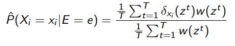
Observe that we didn’t sample from a different $q’(x_i, e)$ for the numerator. Rather, we used $q(e)$ and added some rejection sampling.

Again, we must use the same samples. Because then, if we overshoot, both the numerator and denominator overshoot, which cancels things out.

There is a small problem to this, which is that it’s biased at low values of $T$. In fact, if $T = 1$, the following is true:

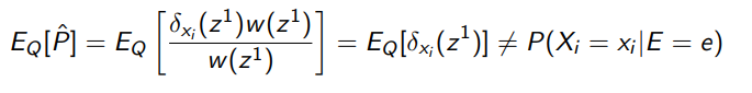
But fortunately, as $T→\infty$, the estimator is asymptotically unbiased. This is because in the long run, the numerator and denominator are both unbiased and so it ends up being OK. However, this is not immediately obvious, but let’s take it at face value for now.