Message Passing

Tags	CS 228Inference

What we have and what we want

We want to have an algorithm that computes marginalization. We did this through variable elimination, which runs in polynomial time in the best case scenario. But this still is pretty bad if we want to do multiple queries. Can we do better?

As it turns out, yes! When we do variable elimination, we cache a lot of intermediate $\tau$ factors. We can use them! But how?

Message passing: analogy with death

Let’s begin with a simple graph $A→B→C→D$ . In this case, let’s find $p(D)$ . We begin by removing $A$ . This requires you to collapse $A$ by computing

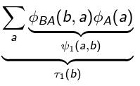
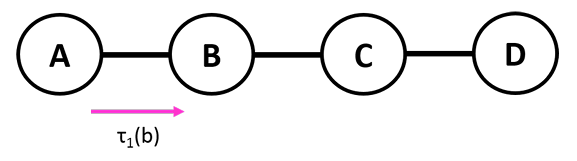
But this is a very nice intuitive explanation! This $\tau$ is the “message” that $A$ passes to $B$ as its dying wish. When it was still alive, the value of $A$ could modulate the value of $B$ . But now that it’s gone, it packages its influence on $B$ into a neat “will,” and $B$ integrates it into its own factor network. In this way, we pass on the message (”legacy”) of $A$ .

You can easily (perhaps a little morbidly) expand this to when $B$ has multiple dependencies (friends). When alive, the friends influence the value of $B$ . But as the friends die off, they leave their last will to $B$ . This $B$ will take each of these last wills and integrate it into its own life as $\tau(b)$ , a joint factor. Because the friends are no longer alive, they can no longer actively influence $B$ . But $B$ keeps the legacy of the friends alive through $\tau$ .

This is perhaps a morbid example but it really helps with the intuition of message passing. Think of it as a “last will”. And as people in line get eliminated, they pass on the influences of their predecessors. Again, as they die, they lose the ability to actively influence the next of kin. But their legacy remains, until we reach the final child. This final child holds its own values, but also the messages (legacies) from all its ancestors. This is what it means to marginalize!

☝

Message passing on trees only work from the leaves up. A node should never pass more than one message. However, because any node can be a root, we have the forward and backwards messages

Belief propagation: introduction

Formally, the creation of a $\tau$ in the process of elimination is known as belief propagation and we have a general formula

m_{i\rightarrow j}(x_j) = \sum_{x_i}\left(\phi(x_i)\phi(x_i, x_j) \prod_{\ell \in N(i) \backslash j}m_{\ell \rightarrow i}(x_i)\right)

Let’s unpack this using our “last will” framework. Who’s dying? $i$ is. Before $i$ dies, it looks at the last wills of its superiors $\ell$ and condenses those together. That’s the product. It considers the relationshpi it has with $j$ , and it smushes it all together into one final product. This is the payload that $i$ uses, and when it finally dies (gets marginalized out), we have one will that is passed to $j$ . Now, this “will” or “legacy” will influence how $j$ behaves because it is a factor $\tau(j)$

Note that if $j$ dies next, this message $m_{i→j}$ is going to be one of the “wills” that it consults in the product. That’s how information is passed!

How many messages are possible?

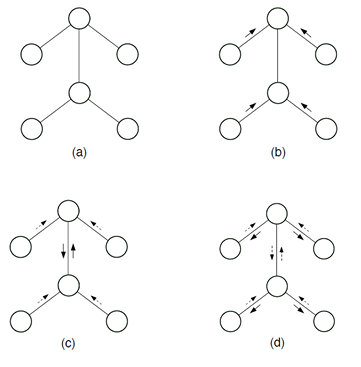
Let’s start by assuming that we are dealing with a tree. Like a family tree, message passing behaves nicely when you are considering information flowing in one direction without a cycle.

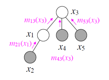
In a graph, one node passes a message to another node. It does this when all of its other nodes have finished passing messages to it (look at the equation above to understand why). Therefore, for every edge, there is two possible messages that can be passed.

And here’s the crux of the problem: given ANY node $x_f$ and all the $2|E|$ possible messages, we can find $p(x_f)$ in $O(1)$ time. This is because

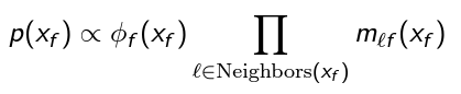
and the $m_{\ell f}$ is precalculated. This is message passing memoization at its finest!

In some literature (and below) we call the product that belief, or $\beta$ . The belief is proportional to the probability.

To calculate the true probability, note that the right hand side produces a new factor. Just normalize the factor!

Message passing protocol

Let’s formalize what we just talked about above. Node $j$ sends to neighbor $i$ when it has received messages from all other neighbors. And again, once this message is constructed we don’t have to do it again. This is how we might build up a message map

To pass a message, you make a joint factor $\phi$ that contains all the children’s message factors (the “last wills”) and the internal factors of the current variable. Then, you sum them over into one $\tau$ that depends on only the current variable. This you send up to the parent as a message. The parent will combine these messages with other messages in a cascade effect.

The neat part is that this can be done in parallel.

Sum-product message passing for factor trees

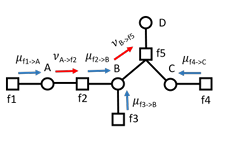
This is another way of seeing everything. We split up a message into two parts. First, a factor-to-variable. Then, a variable-to-factor.

Factor-to-variable happens when you have one factor and one variable. Multiple factors can send to a variable. This is like multiple people can send their “wills” to one person. To accomplish this feat, we must have a standalone factor. This can mean a marginalization

Variable-to-factor is what happens after a factor-to-variable message gets passed. In this case, we need a standalone variable. To do this, we need to combine all the factors into one.

The tl;dr is that FV communication is marginalization because we snip the tail. The VF communication is the product because we need to unify what came before

All communication is done with one variable in mind.

The formalization

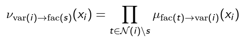
In plain english

Find all the factors that are adjacent to this variable OTHER THAN our target factor $s$ , then take their factor-to-variable product. This factor-to-variable product is essentially combining together their influence over $x$ . This combined influence is what we send down the line to a factor $s$ . The end result is still a function of $x_i$ because again, we are just combining factor influences

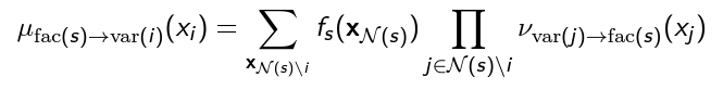
In plain english

find all the variables that contributed to this factor OTHER THAN our target variable $i$ , take their message products

Multiply this with the factor corresponding with all the neighbors of our factor

Marginalize out everything except for our target

The connection

m_{i\rightarrow j}(x_j) = \sum_{x_i}\left(\phi(x_i)\phi(x_i, x_j) \prod_{\ell \in N(i) \backslash j}m_{\ell \rightarrow i}(x_i)\right)

The connection is very strong. So in normal message passing, we do the two-step process all at once so we can essentially just run the factor→variable passing algorithm. By splitting it into a two-step process, you’re essentialy (1) consolidating all messages in the inbox (var to fac) for a single factor for a variable (this is moving from grandchildren to child). Then, you want to find all the children who are contributing, and then sum it together until you just have one factor that impacts the parent. It’s a two-step process but it’s equivalent.

Implementing

You would start with all the variables. Then you send messages to all the factors. If you don’t have an answer, you wait, or you approximate (that’s loopy belief propagation). After all messages have been sent, you iterate over the factors. You send all the messages that are present, and then you repeat.

Why do we do it this way?

This mode of message passing is actually easier to implement in code because factors and variables are typically represented separately.

Loopy Belief Propagation

Why can we do message passing in trees? Well, it has a very nice structure. Information can propagate upwards in the tree very easily. What about a high treewidth graph (i.e. there are loops?)

There are a few primary problems that arise. First, we can’t even find a good place to start the message passing! There are no guaranteed leaf nodes.

To mitigate this, you can use an approximation. Start by defining all messages as a uniform distribution

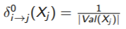
and then iterate through each $i, j$ in the graph until things converge

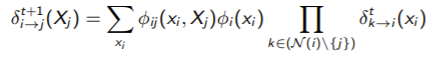
This is not guaranteed to converge and may not settle on the correct marginals. However, empirically, it actually does settle on the right thing

Numerical instability

Because you’re multiplying together factors many times (as opposed to once in non-loopy propagation), you might have numerical stabilibilty issues. To deal with this, you should always normalize all your factors after calculating them. Multiplying by a constant doesn’t change the final marginals because you end up normalizing anyways

Over-confidence

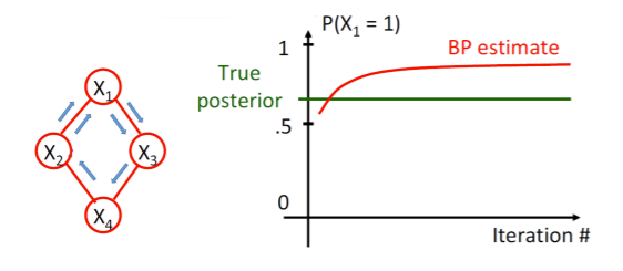
Why? Well, let’s say that $P(X_1 = 1)$ is slightly higher than majority. Then, it influences $P(X_2 = 1)$ to be larger since it has a dependency. And so it propagates in a loop until it reaches $P(X_1 = 1)$ again, at which point it pulls itself up. The tl;dr is that there can be a “Microphone feedback” effect that can lead to double-counting.

When does it work?

When the graph is a tree, belief propagation yields a completely correct answer.

If there is a single loop in the tree, it is empirically shown that it generally converges but it may not converge to the right value.