Motivation

Previously, we looked at inference through a stochastic process. This often involved generating samples from some distribution. In rejection sampling, we essentialy found a way of marginalizing things out. In importance sampling, we found a way of approximating any expected value by using a surrogate distribution.

Now, we still want to sample from a distribution. This particular distribution we can evaluate but not easily sample (sampling requires knowing all values). How can we do this?

Rejection sampling is inefficient, and importance sampling doesn’t work well if the proposal $Q$ is quite different from $P$.

What if we made a shifting distribution that got better every time we ran it, and then at the end, our $Q$ itself is a good estimation of $P$ and we can just use $Q$ directly to sample?

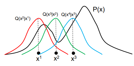
To do this, we have a distribution that depends on its previous value. At each step in the optimization process, it will shift around. It might stay in one place, but in general it will move towards approximating $p$. We will look at how this might be implemented below.

Metropolis-Hastings

Intuition

Suppose that you wanted to find a good present for your friend. You open up Amazon, and then pick a gift at random. Show that to your friend. Now, go to the “related products” section and click on one of the products at random. Ask if your friend likes it better. If he does, then you keep this product and do the same sampling. If not, you go back to the last product and pick another “related product” randomly. Keep on doing this until a certain number of steps has gone by

The general approach

1. Draw a sample from $x’ \sim Q(x’ | x)$. This is your proposed next step

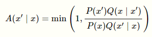
2. Compute the probability of acceptance using the function below

Understanding the $A$.

This is basically how “good” this sample is. You want to bias samples towards “good” samples so that you push closer to $P$.

We can express the inside as something a bit more familiar

Intuitively, this is the quotient of importance weights. An importance weight is larger if the likelihood is higher under $P$, or if it’s rarer under $Q$. So the transitions that boost importance are those that are kept. We will formalize this later.

We note that because we are taking the quotient of products, we don’t need to have normalized probabilities. This allows you to evaluate MRF’s efficiently!

Understanding $x|x’$ and $x’|x$

Basically, $x, x’$ are two samples. You should not think about them as “before and after”, because that can be confusing as $x|x’$ is like moving back in time.

As an example, if you let the $Q$ be a gaussian centered around the past sample, then $Q(x| x’) = Q(x’|x)$ because the distribution is symmetric (i.e. if $x$ and $x’$ are two posts in the sand, it doesn’t matter if you stand at one post and look at the other post, and vice versa. This actually simplifies the acceptance probability.

The algorithm

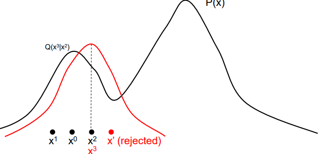
While the samples have not converged (burn in)

1. $x’ \sim Q(x’ | x)$

2. If $u < A(x’ | x)$, let $x = x’$

3. Else, let $x = x$.

After a while

1. Sample from $x’ \sim Q(x’ | x)$ where the $x$ is seeded by the end of “burn in”

This works because the as you keep on running the burn-in, the distribution evolves until it fits the distribution.

Why does MH algorithm work?

(note: this requires content that we don’t discuss until later in this document)

In MH, we define

Here is the crux of our argument

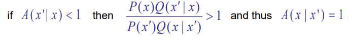
Basically, if you flip the before and after, the quotient becomes greater than 1 (the numerator and denominator differ by just an inversion of $x, x’$)

From this observation, we get this derivation (note how the flip is used on the fourth line)

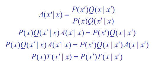
And this is exactly the detailed balance condition!

Gibbs sampling

This is actually just an MCMC algorithm with a very simple implementation for graphical models. It helps us sample from any sort of graph

The intuition

This is much like how writing feedback works like. You will read a draft, and then you might make a small modification. Then, you give the whole thing another read, and then you might make another modification, etc. Each time you do a read, you will make a small modification conditioned on the rest of the creation. .

The method

Suppose that the graphical model has variables $x_1, ..., x_n$

1. Initialize $x_1, ..., x_n$

2. Do until convergence
   1. For all variables in $x_1, ... x_n$
      1. Sample $x\sim p(x_i | x_{-i})$ (where $x_{-i}$ are all the other variables)
      2. update $x_i \leftarrow x$

This would be the burn-in process. During the sampling process, you would literally do the same thing but this time you keep the $x$ assignments that come out as samples.

Why does this work?

Well, it comes down the markov blankets. When you observe everything and sample one variable, it is easy to sample. For MRF, you would just consider the neighbors. For Bayes, you consider parents, children, and parents of children

Connections to MH algorithm

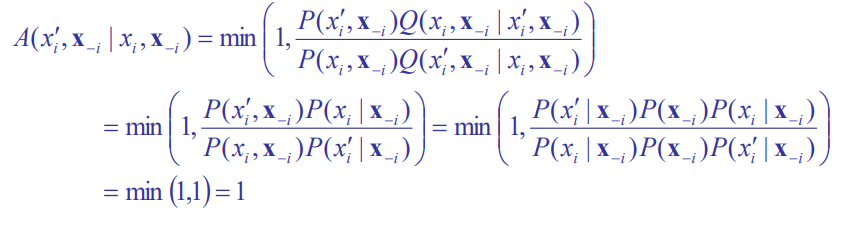
As insinuated before, Gibbs sampling is just a special case of MH in which

This is how you sample the next step. Note how you keep everything constant except for one variable. Now, we can plug this into $A$ and get the following through chain rule:

Markov Chains

If you are looking to implement things, then we’ve talked about everything there is to know. However, the cooler part of the algorithm is the Markov Chain framework. Now, buckle tight because we are about to deal with some weird things!

The key insight is that we are not training anything. The Q is a distribution without any modifiable parameters, other than the previous state it was in. As such, we are just encoding the evolution of the sample in the state of the algorithm.

The construction

This reminds us about the markov chain, in which the transitions to next states are dependent ONLY on the current state. Let’s try to construct this.

Say we had $n$ variables. Let each node be an assignment to the variables. So if the variabes were binary, there would be $2^n$ nodes. To run MCMC, you would

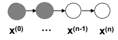
1. Start at an arbitrary starting node

2. Follow the transition probabilities. At each step, you will do something in the node. If you reject the change, it’s like going on a self-loop. If you accept the change, it is like moving along an edge.

The magic part of MCMC is that we implicitly construct the markov chain, which is good because the chain requires an exponential number of parameters.

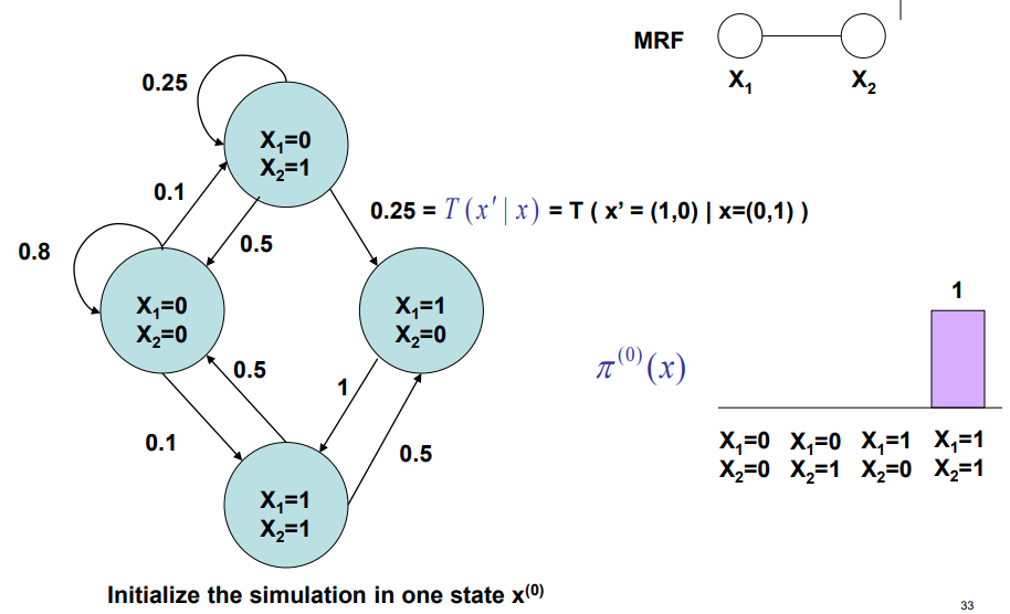
Chain sampling

We call this process a markov chain sampling , and we can express the outcomes as a directed network

Now, this is DIFFERENT than the original model (in the examples above, it is just two variables connected by a single edge).

The distribution across each variable, $\pi^{(i)}(x)$, represents the distribution across different simulation runs. Here’s a way to help you understand. When we run the sampling step, it’s as if we are setting a little grasshopper free on the chain. After it burns-in (stabilizes), the grasshopper chooses its next node as if it were sampling the next node from the original $p$.

However, when we look at $\pi$, we are looking at a whole population of grasshoppers hoppping around, and you generate a historgram of where they are. This is what the distribution comes from.

To reiterate (because this is not obvious) a single MCMC algorithm iteration generates samples from a distribution that approaches( the desired distribution. If we run a lot of these MCMC algorithms, you will get a distribution of samples across each step, which becomes an estimation of the distribution it’s sampling from, which again, is shifting.

Stationary Distributions

The different distributions $\pi^{(i)}$ are related through a transition kernel $T(x’ | x)$, which is basically the edges on the Markov Field

You can think of transitions as the conditional distributions, so you end with a joint distribution of $x, x’$ that you remove the “old” $x$ from.

The limiting distribution $\pi$ is defined as

So basically it’s the distribution we end up with after running the transition for an arbitrarily large number of times.

We define a stationary distribution as the following:

A limiting distribution is a stationary disribution because if you add more $T$ to the $T^\infty$, the distribution doens’t change (infinity plus one is also infinity)

Conversely, a stationary distribution may NOT be a limiting distribution. A limiting distribution is a stricter restriction, in which we want all possible initial distributions to converge to one $\pi$. On the other hand, a stationary distribution just states that one distribution doesn’t change when the transition is applied. For a transition to be well-defined, it has at most one limiting distribution, but it can have multiple stationary distributions. Subsets of starting distributions end up in each stationary distribution.

When a stationary distribution exists, we can keep on sampling and get the desired distribution. Our goal is to show that this exists and that it converges to the desired distribution. Again, resampling just means running another iteration of the MCMC iteration. There is NO training going on!

Achieving stationary distributions

We need two conditions for stationary distributions.

First, the distribution should be irreducible, meaning that you can move between any two states with non-zero probability in a finite number of steps. This means that you can’t have any “death” steps like shown below. (it’s called irreducible because a death state is “reducible”)

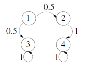
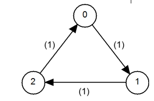
Second, the distribution should be aperiodic, meaning that you can return to state $i$ at any time. This is just the “no circle” restriction of markov chains, which prevent you from just moving continuously without settling on something. A classic example is $T = \begin{bmatrix} 0 & 1 \\ 1 & 0\end{bmatrix}$, which constantly oscillates. We also show an example below.

We define ergodic (or regular) as markov chains that are both irreducible and aperiodic.

Why do we care?

Well, the following statements are equivalent

1. The chain is ergodic / regular

2. There is a stationary distribution

3. There is a limiting distribution

This means that regular chains have one distribution that doesn’t change when you apply the transition

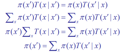
Reversible (detailed balance)

We can show ergodicity by showing that we can “reverse” the distribution by applying the transition operation.

This is not news; you can actually easily reduce this down to the definition of a stationary distribution

Slight nuance

Samples from a markov chain are NOT independent because they are drawn from samples before. However, they are an unbiased estimation of the distribution.