Recap

Making a model

We want to make a model $\hat{p}$ that matches the target distribution $p^*$ as much as possible. To do this, we maximize the DKL, which becomes

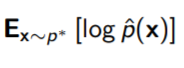
because the first component is just entropy and it doesn’t matter because $\hat{p}$ is not included. So it is accurate to say that we are maximizing the expected log likelihood of the trial distribution WRT the target distribution.

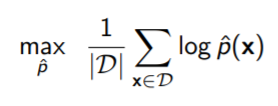
We don’t have $p^*$; rather, we have samples from it. So we estimate using Monte Carlo, which yields

Optimizing bayes nets

Now, for Bayes Nets, we took the expression above and recognizes that the network factors into the CPDs, and that we can take the summation across the dataset and turn them into “counts”

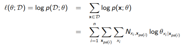
You can show that the bayes networks have a closed form solution. We can compute this because the objective decomposes by variable. We took a look at this in a past section.

What about MRF?

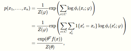
The objective becomes

Note how we always love to work in log domain because the products turn into summations. Note that, unlike the Bayes setting, the MRF doesn’t decompose perfectly. It has this nasty $Z$ term that isn’t defeated with the log function.

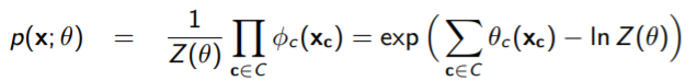
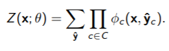
Regardless, we do have some degree of decomposition across each clique. Now, what exactly is this function $\theta$? Well, why don’t we rewrite it as this, where we sum across all values of $x_c$ (which we denote as $\bar{x}_c$).

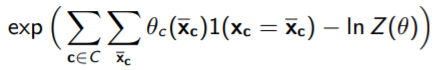
Now, you can start thinking of $\theta_c$ as being conglomerated into a large $\theta$ table, in which you have values for all $x_c$ across all $C$. We did this last time with the framing of MPE inference as a linear programming algorithm. Therefore, you can see this whole thing as being

Now, here’s the rub. The normalization constant factors into the optimization, so we can’t ignore it. Intuitively, this is because unlike the bayes optimization, $\theta$ has no constraints that they have to add up to 1. Instead, the larger we make $\theta$, the larger we make $Z$. Unfortunately, the $Z$ does NOT decompose over terms, so it becomes more complicated.

Furthermore, we can’t even compute $Z(\theta)$ without using some form of inference over the model, and that can have exponential complexity.

We are forced to resort to a gradient based approach.

The gradient of $\log Z$

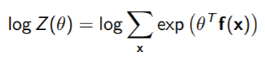
So we must take the gradient of the whole $p(x)$ WRT $\theta$, but to even see if that’s feasible, let’s take the gradient of $\log Z$. This is a traditional log-sum-exp structure

We use a simple chain rule:

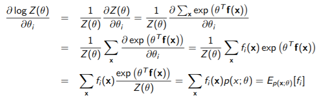
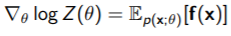
This yields a pretty nice solution. The last step uses the insight that $\exp(\theta^Tf(x))/Z(\theta)$ is just the original distribution.

Therefore, the full gradient is just

And this part is really cool: you can actually show that the log-partition function’s hessian is just the covariance of $f(x)$, which means that log-partition function is positive semidefinite

• Proof

  

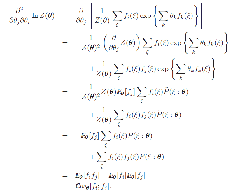
The key upshot is that $\log(Z(\theta))$ is convex (bowl) so $-\log Z(\theta)$ is concave (mushroom)

Putting it together

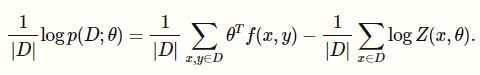
If we have

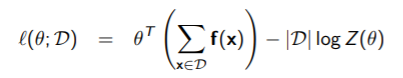
(the $|D|$ comes from moving the log-partition out of the summation), then we can take the gradient. The first part has a simple gradient: $\sum_Df(x)$, and the second part we have already derived.

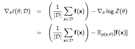
(this is shifted by a scalar $|D|$ for pedagogical purposes)

Intuition

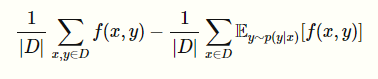
Because this is a concave function, we can just set the elements equal to zero. But what does that mean?

Well, recall that $f$ is the sparse 0-1 vector of assignments that takes in a vector $x$ and outputs this sparse vector. The $\sum_D f(x)$ is therefore a monte carlo expectation:

So we are just trying to match the expectation of assignments (read: data points) from the sampled distribution with our constructed distribution! Neat!!!

This is known as moment matching, and it’s shared in many different techniques

Actually doing this

Well, gradient ascent requires marginal inference because we need to calculate $p(x)$, which has the partition function. This is hard!!

To get around it, we use approximate inference. We estimate $E_{p(x)}[f(x)]$ using a technique like gibbs sampling. How? Well, our goal is to sample from $p(x)$, which is generally intractable due to the partition function. But in gibbs sampling, we can sample from the markov blanket, which make the partition function over one variable. So, at the end of the day, you have a bunch of samples generated from $p(x)$, which you can then use to approximate $E_{p(x)}[f(x)]$.

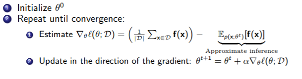
So here the algorithm:

Brief aside on exponential functions

Recall from CS229 that this formula, $\exp(\theta^Tf(x))$ is an exponential family of distributions. This is log-concave in their natural parameters. The vector $f(x)$ is known as the vector of sufficient statistics, which parameterize some distribution. This is a function of $x$, which is why different values of $f$ yield different distributions.

Other approaches

So we just went through a derivation that shows you how we might be able to learn MRF directly. More specifically, we needed to sample from $p(x)$ which was very difficult so we used Gibbs sampling. But can we use other approximations that maybe makes our lives easier?

Pseudo-likelihood

By the chain rule, we can factorize any distribution as

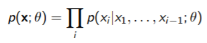
This doesn’t help so much because it doesn’t respect the structure of the MRF. But what if we made it respect the structure??

We can approximate the joint by doing

Here, $N$ is the Markov Blanket. Intuitively, you’re assuming that $x_i$ depends mainly on its neighbors because we cut things off at the markov blanket. This allows you to compute each marginal easily because the partition function is over one variable.

Therefore, the average log likelihood can be replaced

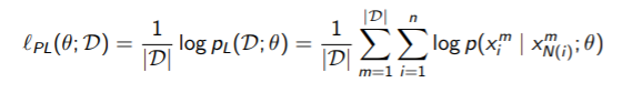
The key upshot here is that we’ve separated each component (which had to do through cliques, not individuals, before).

To be more precise, our original decomposition of the likelihood relied on the factors, which meant that you need the partition function over the whole distribution. Now, you are saying that we can factorize the distribution into smaller true distributions (not factors). These we can calculate by marginalizing over one variable only. If we had a pairwise MRF, then we can get

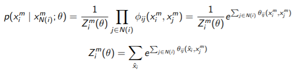
It looks ugly, but it’s tractable. We can compute the derivative and maximize without using any approximate inference techniques. With large enough data points, the parameters derived from pseudolikelihood will approach the true parameters.

Again, remember that the parameters are just a table.

Learning Conditional Models

Recall that a conditional random field is VERY similar to an MRF, just that the partition function depends on the conditioned variable

In some cases, if $y$ is very small, then this $Z$ is tractable.

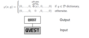
The feature function $f(x, y)$ are still indicator functions, but now they take in two parameters instead of one. They function in the same way though.

Our objective

Instead of finding the distribution that best explains a dataset, you want to find a conditional distribution that best explains a dataset of tuples. You want to find a good $\theta$ that captures the relationship between $x, y$.

We do the same calculations and we get that the gradient is

However, unlike the MRF, the $Z$ can’t be computed once. This is because you need to find $Z(x)$ for every point. Now, for Gibbs sampling, this doesn’t change too much because you don’t explicitly compute the partition function anyways.

Structure matters

To close, let’s look at a handwriting example. We want to compute $p(y|x)$ where $x$ is an image and $y$ is the prediction. We might start with this structure

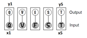
Now, this is pretty good because the inference on $Z$ just cycles through $26$ values of $y$ each. But this doesn’t use any information about the inter-character relationships. Can we do better?

Hmm. So now we’ve reduced it down to one model, but now we must check $26^5$ different values, and that’s pretty bad.

Compromise?

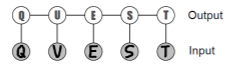
Inference here is approachable because it’s a tree! And we also take into account the intercharacter relationships!