Quick recap

1. To perform inference, we need to marginalize out variables.

2. We can do singular inference through variable elimination

3. To find marginals in constant time, we use a bunch of variable elimination in what we call message passing

Junction tree algorithm

Previously, we looked at message passing in graphs. It works all the time on trees but only occasionally on loopy graphs. Is there another way?

Intuitively, this algorithm will break the graph into clusters of variables such that between the clusters, the graph behaves like a tree.

Clustering variables

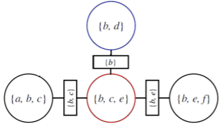
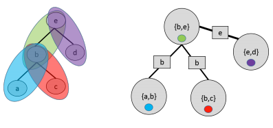
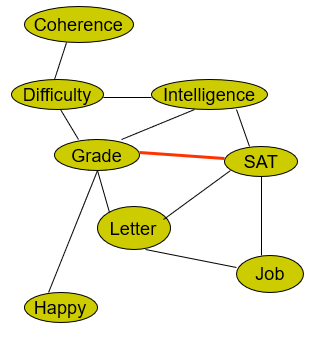
Suppose we started with this graph

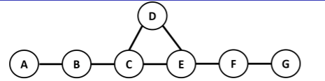
We can turn the center clique into a new variable $w$ by defining an equivalent joint distribution

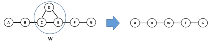
Due to the graph structure, we can let $\phi_{BW}(b, w) = \phi_{BC}(b, c)$, $\phi_{WF}(w, f) = \phi_{EF}(e, f)$ and $\phi_W(w) = \phi_{CD}(c, d)\phi_{DE}(d, e)\phi_{CE}(c, e)$

In other words, this $W$ is a proxy that we can operate our belief propagation on, and when we encounter factors like $\phi_{BW}$ we replace it for what it actually stands for.

Clustering multiple

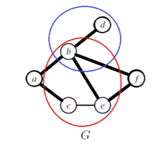
When you want to make multiple groups, you need to pay careful attention to the intersection between the clusters. This is because these are variables that are being pulled in different directions by each cluster.

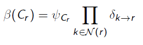
More formally, these variabes are known as separator sets or sep-sets defined as $S_{ij} = C_i \cap C_j$. When constructing the cluster tree, we use boxes on the edges to denote this

Preserving families

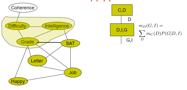
Now, here’s another important thing we must consider. When clustering, each factor’s scope must be contained within some cluster. This has intuitive meaning because we want to do internal calculations inside each cluster.

We have a nice color-based visualization that shows how the factors are perserved

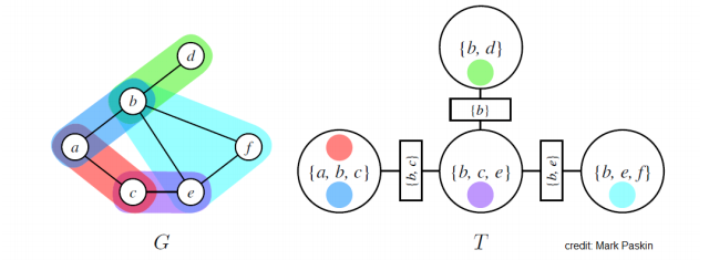
When family is preserved, we call this tree a cluster tree.

Joint distributions in trees

With family preservation, you can just define the joint distribution as

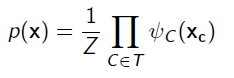
where $\psi_C$ is a potential for each cluster. This is legal because you can just multiply together all the $\phi$ that are part of the cluster to form a larger factor $\psi_C$.

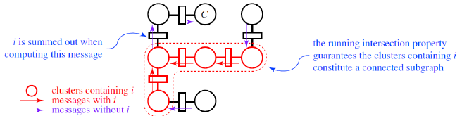
Running intersections

Another important feature to have in these cluster tree is running intersections. Any pair of clusters may be connected by nodes in common in the original graph. We denote this as $V\cap W$. In the cluster graph, we must also keep this connection, meaning that for every pair of clusters $V, W$, all clusters on the path between $V, W$ must contain $V\cap W$

Perhaps we can better understand this through a negative example

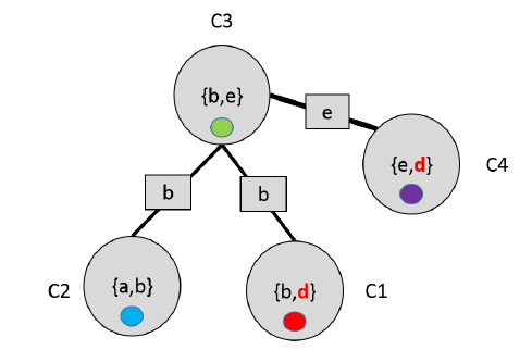
In this case, the $d$ is present in both $C1, C4$ but $C3$ does not have it. Intuitively, this is illegal because both C1 and C4 have $d$ and so they need to be consistent with each other, and yet they have no way of communicating the $d$.

These requirements, reviewed

If any of these requirements are not satisfied, then it is not a junction tree

1. Tree. We need natural order for belief propagation

2. Family preservation: we can assign factors to clusters without splitting things up.

3. Running intersection: clusters with variable $X$ are connected, so we know that once it stops appearing, we are safe to remove the variable.

Inference on Junction trees

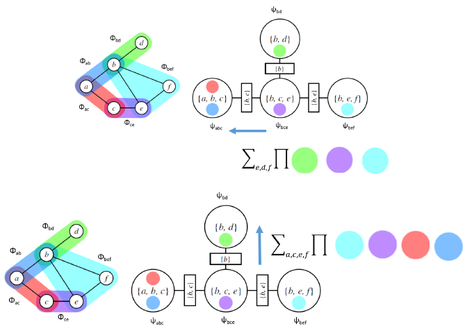
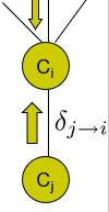
At the most basic level, it’s just message passing between the nodes. Each cluster sends a potential function to each neighbor, and each cluster will aggregate all messages before sending it upwards.

In normal message passing, we a message from $A→B$ would pass a factor $\phi(B)$. However, in junction tree message passing we pass a factor that includes all the elements in the sepset. That’s the difference.

Formalism

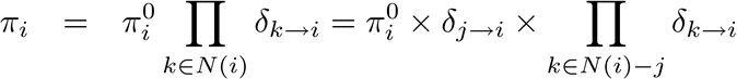
This is where the sep-set comes in. When we send a message upwards, we marginalize out everything that isn’t in the sep-set. Intuitively, this is because the parent node doesn’t get direct influence from variables that are outside the sep-set in the child node. Mathematically, it looks like

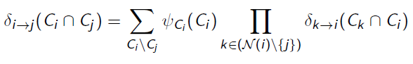
The outer summation removes the sep-set and the parent set, and the inner product take the joint factor across all the children of the current node.

If you look at the junction tree for a tree, you will see that this message passing algorithm is just a general case of the tree message passing algorithm

• Great visual

  

The final marginal

The probability of the cluster is just the final product

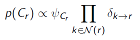
And from this point we can just marginalize the elements of the cluster until we get our desired variable. If the variable is present in multiple clusters, you can choose either one. When the messages are done, we call the tree to be calibrated and the belief is just

Making Junction Trees

We can make a degenerate junction tree from any possible graph, where the whole thing is in the cluster. This is counterproductive because message passing would be exponential in complexity.

From a tree, we can also easily make a junction tree

Variable Elimination and Junction Trees

As it turns out, we can easily use variable elimination to make a junction tree.

1. Get your elimination order

2. for every variable to eliminate, the clique you form during elimination is a clique in the Junction tree

3. The clique that you are left over, after marginalizing your eliminated variable, this is the shared separator sets. You can imagine an edge as a factor that involves these variables. Therefore, this edge should go to any cliques that are later formed that use this created factor. Multiple edges can go “into” a node but only one can “leave”. It’s in quotations because it’s technically undirected. However, because there is only one parent, we can say that it is a tree.

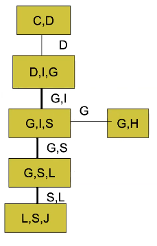
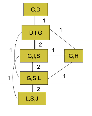
Hmm. This seems confusing. Can we clear it up a bit? Let’s look at an example. We want to eliminate in the order of C, D, I, H, G, S, L. We start with

We eliminate the first two variables as so

Note how the circled object includes the D that we want to remove, but the clique is added and the remaining variables get passed down the line. It is connected to the first clique because the induced factor $\phi(D)$ is used during the construction of the next clique.

Now, you don’t necessarily have to build down the tree sequentially

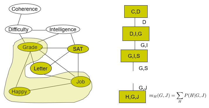
Here, we don’t use any existing cliques so we start anew.

We also see that a clique may take multiple induced factors

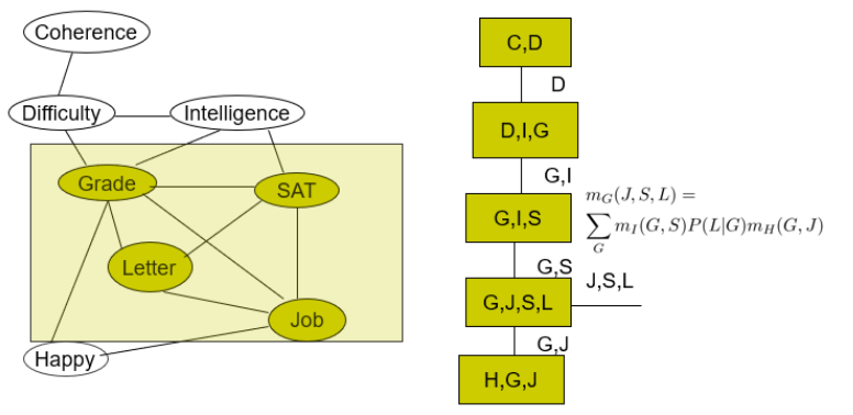
We can remove cliques that are not maximal, i.e. cliques that are strict subsets of other cliques in the clique tree. These we can group together.

As a side note, if you have a bad VE ordering, your cliques will become very large, which is not good for the junction tree.

Complexity analysis

We first must make the tree (compilation) and then we must propagate the information (propagation).

Compilation is polynomial time given an elimination ordering.

Propagation is limited by marginalization. It’s exponential to clique size, and more specifically, the size of the largest clique.

Extras

Message passing with division

Let’s look at how messages relate to each other

The calibrated potential at $C_i$ would be

where $\pi^0$ is the original factor of the clique. The message from $C_i → C_j$ would be

The $C_i - S_{ij}$ is just anything that is in $C_i$ that is not in the separating set. This, of course, needs to be marginalized out.

if we take the first equation and express the $\prod \delta_{k→i}$ in terms of $\pi_i$, we get

And why do we care?

Well, note how the division is symmetrical. If you flip $i$ and $j$ (i.e. compute $\delta_{j→i}$, you would only need to flip the messages and the $\pi_i$ into $\pi_j$.

Lauritzen-Spiegelhalter (Belief Update) algorithm

1. Each cluster maintains fully updated current beliefs $\pi_i$. These include the messages passed from neighbors

2. Each sepset $s_{ij}$ keeps some $\mu_{ij}$ that is the last message passed between $C_i, C_j$

3. Any new message passed between $C_i, C_j$ is divided by $\mu_{ij}$

Uh, why the hell does this work? Actually, so this answers many of our questions on how belief propagation is actually implemented. The variable “fires” when all but one of the the neighbors give the message. But in reality, it’s better to wait until you have ALL the messages going one way, and then fire everywhere at once. However, we encounter a problem. When we fire, we want to have a factor that includes all variable messages BUT the target. So we can’t just send the same message to everyone.

However, we note that if we create this $\pi_i$ which is the calibrated factor that has all the messages collected, it is related to the last message through the quotient (see above). Therefore, we can send a generic message to all neighbors as long as the edges between them keep track of the last message.

The tl;dr: with the LS algorithm, we can wait until we’ve received all the relevant things, and then we can send a generic message to all the neighbors and have the edges figure things out.

There are some nuances that we won’t worry too much about, like how the propagation is started. Just know that there is another way of doing things!

Junction Trees from Chordal graphs

Instead of VE, we can also use a chordal graph. What is a chordal graph? A chordal graph is a graph whose largest possible cycle is 3. You might be able to find longer cycles, but there are edges that make it shorter that you can take. Perhaps it’s better if we learn from example

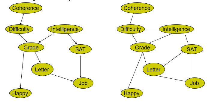
we start with the original bayes network, and then we moralize it. Next, we make a Chordal graph. Here, the only edge we add is

Now, what’s so special about this? Well, we can just cluster the graph. This can be done arbitrarily. Just pick things off and cluster them! The largest clique is necessarily just 3 elements large.

Then, you get something like this

You give weights to how many nodes they share in common. And then, run the maximum spanning tree algorithm! You want the highest summations of the weights because the higher the weights, the less you eliminate per marginalization (think about it for a hot sec). Then, you get this!