The big idea

Given that we have previous knowledge of a latent variable structure, can we infer the parameters from the data? It turns out that we can, using a sort of coordinate descent approach!

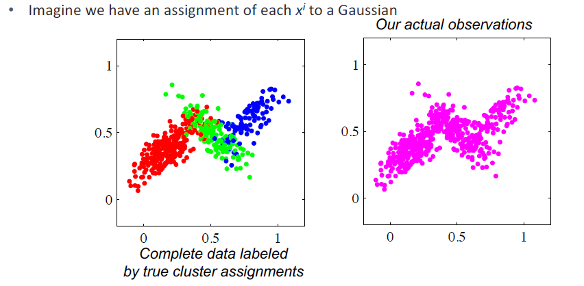
Partially observed data

If you had $p(X, Z)$ and $Z$ was not observed, you have a partially observed problem. This can be when $Z$ is a latent variable, or it might be that you have a noisy data channel and some bits you just don’t know. It might also be if you had partially supervised data, in which you had a lot of unlabeled data and a few labeled examples.

We’ve learned Bayes networks and MRFs. Now, we will look at methods to learn partially observed data. The EM algorithm works on bayesian structure and MRF, though bayes networks have simple solutions.

What do we want?

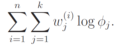
We want to maximize the log marginal likelihood

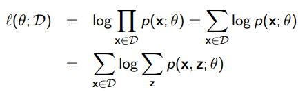
Here, because there is a sum in the log, there is no longer a closed form solution like we had in the fully-observed Bayes network. This is because the marginalization $\sum_z$ is summing across all values, which requires inference. Of course, this can be exponential in complexity.

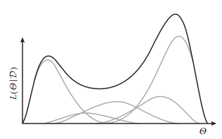
Another intuition is that the $z$ can add complexity. Each point given $z$ might be a simple distribution, but when we marginalize, we can get a multimodal distribution

To do this, we use the EM algorithm. The big idea is that we “hallucinate” the true values, and then we update the parameters based on the completed data.

The intuitive setup

1. Assign values to the unobserved variables

2. use inference to figure out its likelihood in the joint distribution

3. Weigh the datapoints in accordance to how likely they are to occur. Essentially, you’re like generating new datapoints that are weighted in importance depending on what the model already thinks is true.

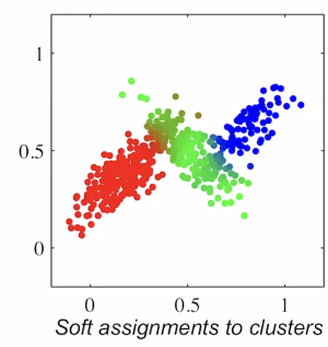
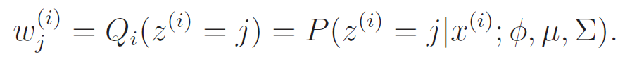
E step

Now, let’s formalize this a bit.

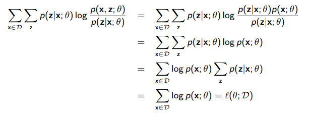
Basically, we want to see the distribution across $z$ of each $x$. This is calculating

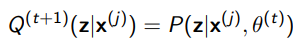
We are assuming that we have access to the joint distribution. We technically only get data from the environment, but let’s think inductively: say that we are given a decent joint distribution. Can we calculate $p(z | x)$? And the answer is yes!

Well, for the most part. In the EM algorithm, we assume that $z$ is a “selector” variable that has only a few possible values. For example, in a mixture of gaussians, it would just be the selected gaussian. If this were not the case, then the E step might be hard to compute.

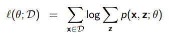
M-step

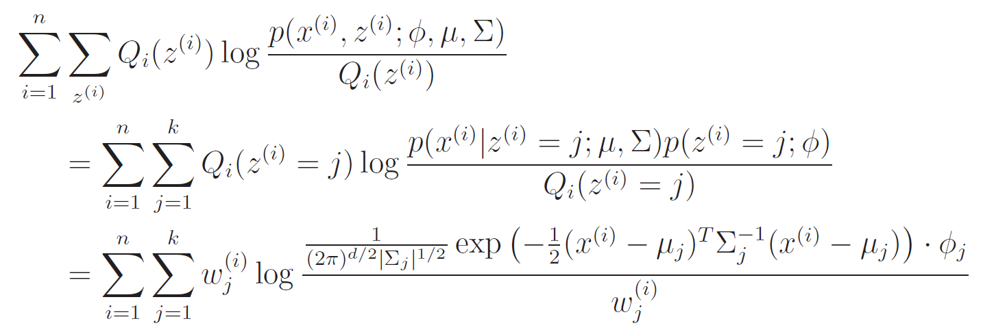
The marginal log likelihood is this

Well, we can try to turn this marginalization into an expectation through importance sampling

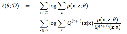
Now, we can use jensen’s inequality to flip the log and the summation, because the log of an expectation is greater than the expectation of a log (think of the secant line as the expectation and the curve as the log)

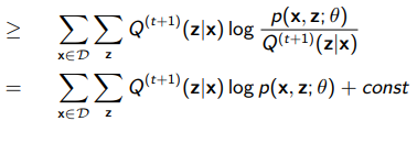
What have we done?

We’ve created a lower bound, where

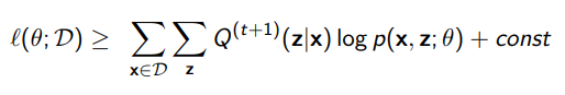
If we are smart, if we optimize the lower bound, then the likelihood must follow.

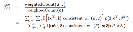
If you actually do the math, you will see that the optimization is just a weighted counting. In other words we consider the hidden variable as part of our counts, but we weigh it with the likelihood that the hidden variable happens

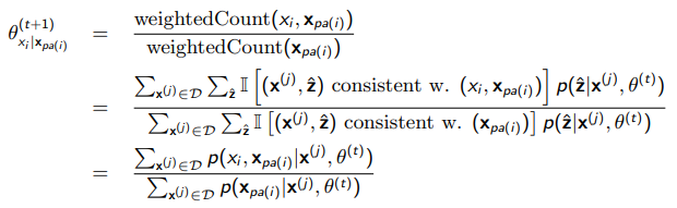
If you are still struggling, you can think about taking a data point, making $n$ fully-observed data points from it (one for every possible $z$, and then weighing them by how likely they are to occur.

What $Q$ to use?

To repeat, we use the following. Why though?

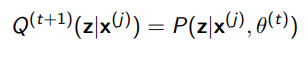
Well, when $Q$ is this, the lower bound is tight. In other words,

But why does this matter? Well, because of one simple reason. Think about the lower bound as a pool floor, and think of the likelihood as a person swimming. The person can’t possibly go below the pool floor, but if the water is deep enough, the pool floor can be risen without the person rising. However, if the person is touching the pool floor, then the person must rise when the bottom is risen.

This is exactly the deal with the lower bound. If we attempt to optimize the lower bound when it’s not equal, then you might not touch the likelihood at all. However, when it’s a tight bound, you are guaranteed to increase the likelihood.

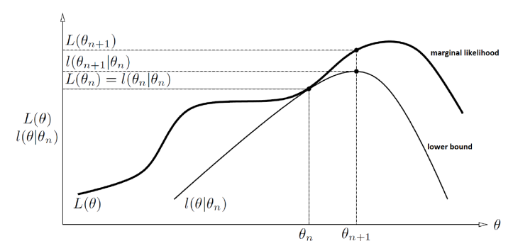
Why is this bound tight?

Well, that’s a simple matter of algebra

Another justification

Here’s another reason why we use $q$ the way we do. When we started with the EM algorithm, our overarching goal is to optimize for $\log p(x)$, which we have rewritten using jensen’s inequality as

Now, in our M step, we split up the $p(x, z)$ into $p(x | z)p(z)$, which is totally valid. But we can also split it up into $p(x)p(z | x)$, which gets us

The first term doesn’t depend on $q$, and the second term is just DKL, so we get that

Our goal is to optimize the left hand side, but we have to optimize the right hand side because it’s tractable. When we modify $q$, we can only change the KL divergence component. And ideally, we want to keep on pushing the lower bound up, so this is why we minimize the divergence and make $q(z) = p(z | x)$. This is a lot of mathematical gymnastics, but it shows yet another reason for $q$ being assigned the way it is. This is also another justification for pushing the “gap” in the lower bound as close as possible through the choice of $q$.

Properties of EM

1. Parameters that maximize expected log-likelihood lower bound can’t decrease it, because it’s equality.

2. EM can converge to different parameters and can be unstable

3. You need to do inference on the Bayes network during the E step

Alternatively, you can do gradient descent on marginal likelihood, which is kinda like coordinate descent.

Mixture of Gaussians (example)

We have a distribution

Which has $X \sim \mathcal{N}(\mu_y, \Sigma_y)$. In other words, $X$ is a mixture of gaussians. We assume that there are $k$ gaussians; this is a hyperparameter.

We have three parameters: $\phi, \mu, \Sigma$. The $\phi$ is the prior on the $z$ distribution, such that $p(z_j) = \phi_j$. The $\mu$ is the mean vector of the distribution, and the $\Sigma$ is the covariance matrix.

E-step

The e-step is pretty easy, because we just sample the posterior distribution of what we have right now

to do this, you use bayes rule: $p(z | x) = p(x | z)p(z) / \sum_z p(x | z)p(z)$

The M-step, $\mu$

In this step, we just need to maximize the expectation:

We can take the derivative of the $\mu_j$ and set it equal to zero. This is nothing new, but it's an algebraic hardship

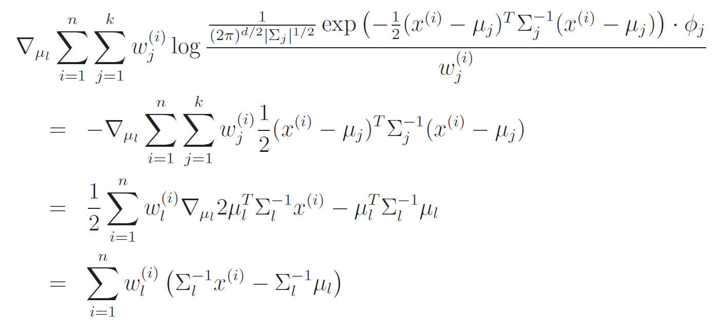
We can set this equal to zero and solve like usual

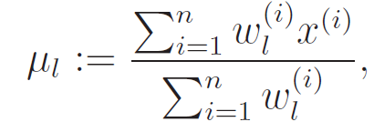
Note how this is SO similar to what we did for the GDA! We just have a "soft" weight now.

M-step $\phi$

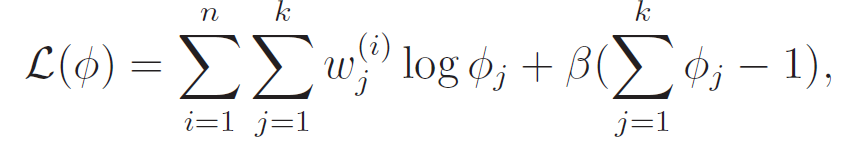
This is the prior, and we we can optimize it with this objective

However, we are constrained by $\sum \phi = 1$. therefore, we can set up the legrangian

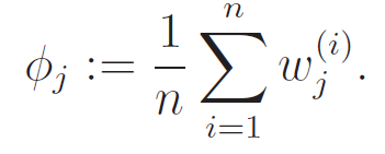
This we can easily set to zero and solve, getting us

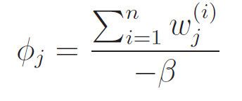
Because $\sum w_j = 1$ and we have the constraint that $\sum \phi_j = 1$, we can easily derive that $\beta = -n$. As such,

The M-step, $\Sigma$

In general, as you have seen, the M step of the algorithm uses the same steps as GMM derivation, but instead of an indicator function that selects for $1\{z = 1\}$, we have a soft distribution. However, in the eyes of the calculus, the constant doesn’t matter. So the form is the same, and we get

Intuition of the M step

From this GMM derivation, we can get a sort of intuition for how we can run M step in general.

1. Formulate an optimization equation in which you are given all the labels you need

2. Now, soften it. Create a weight that represents the likelihood of this label occuring given your current belief distribution.

Example

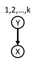
Suppose you had $y → z →x$ and you wanted to construct the M step, where $x \sim N(\mu_z, \Sigma_z)$ and $p(z | y) = \lambda$ if $z = y$ and $1 - \lambda$ if $z \neq y$.

1. To optimize $x$, we note that in the hard optimality, we just need to select the datapoints that have the required $z$ and then run a standard gaussian optimizing objective. So in the soft optimality, we just need to compute $p(z | x) = \sum_y p(y, z | x)$.

2. To optimize $z$, we note that in the hard optimality, we just need to count the number of times $z = y$ in the data. In the soft optimality, we just need to compute $p(z = y | x)$, which can be done using the joint distribution (i.e. $p(z = 1, y = 1 | x) + p(z = 0, y = 0 | x) ...$

3. To optimize $y$, we note that in the hard optimality, we just need to count the number of y’s in the data. So in the soft optimality, we just need to compute $p(y | x)$.

The moral of the story is this: in the M step, think hard, but operate soft!

Additional content

K-means as EM

K-means is actually an GMM algorithm with two constraints: spherical gaussians and hard assignments. If we do hard assignments, then we get that

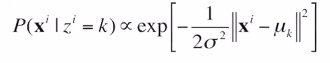
and everything else is zero, so the summation drops out. The E-step then becomes a simple assignment based on distance.

The M step is exactly the same as the K-means, because $\exp$ is monotonic, negating a maximization becomes a minimization, and scaling by $\frac{1}{2\sigma^2}$ does not change anything.

As such, we get

like before.