Why this?

Well, this is the probabilistic interpretation of neural networks. So it has some pretty neat theory!

This is not suited for normal backpropagation

• slow for multiple hidden layers (less important now)

• unlabeled data

• stuck in poor local optima

Boltzman Machines

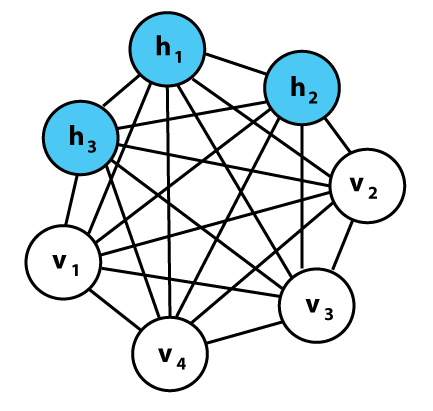
This is just an MRF that has some elements observed and other elements latent. This is an easy model but very hard to compute samples or learn.

• sampling: use gibbs sampling or other MCMC methods

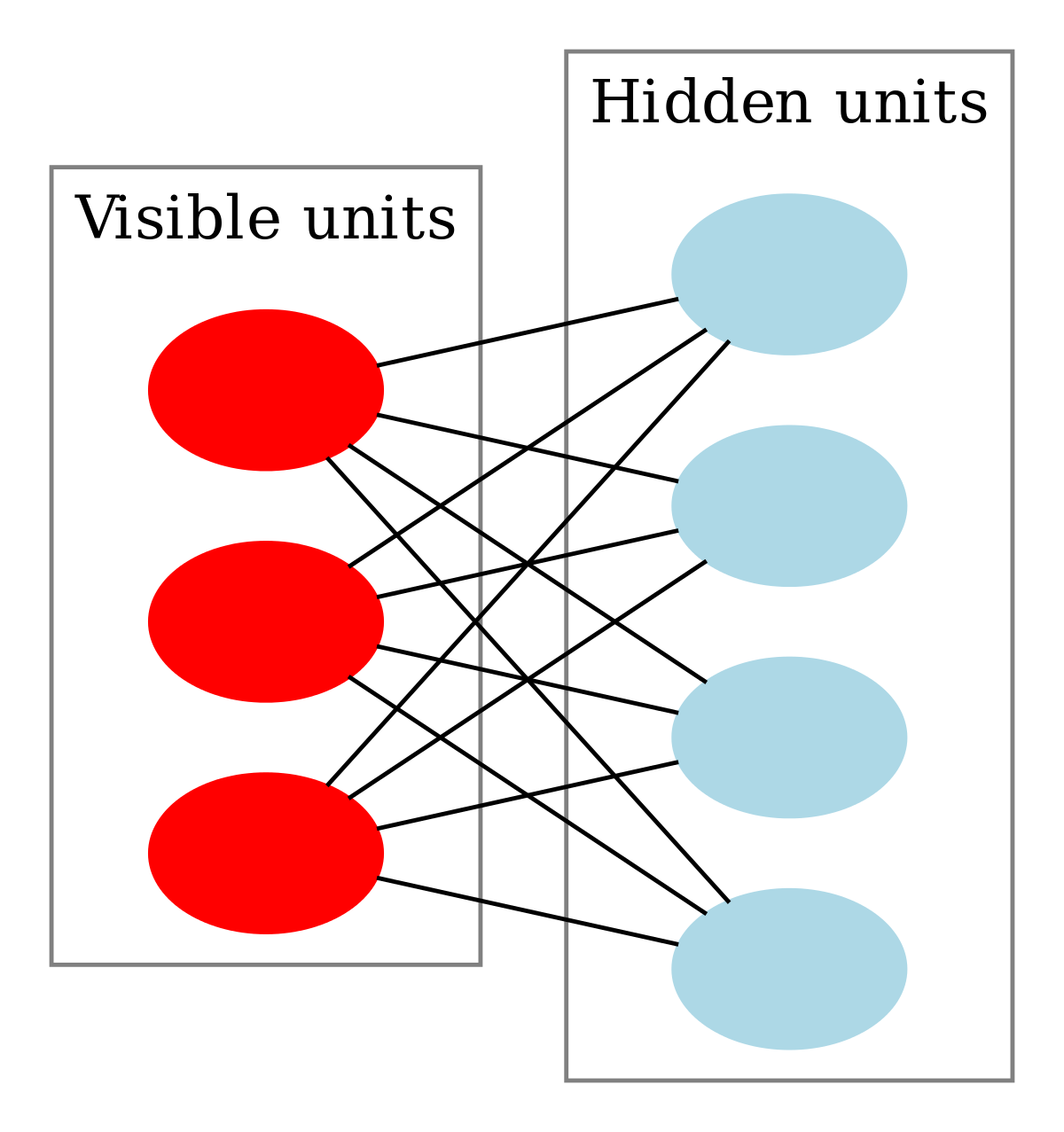
If we restrict the connections, things are a bit easier. A restricted boltzmann machine has one set of observed units that are fully connected to a set of hidden units (which are not connected themselves).

This is different from deep belief networks because DBN are directed. Usually these belief networks are binary.This makes the problem a bit easier.

Deep Belief Networks

• Easy to generate visible effects due to causality

• Very hard to infer hidden causes due to “explaining away”

• We need to infer the stochastic hidden causes from the visible effects to do any sort of optimization, so therefore learning the parameters is also hard

Learning from posterior distribution

So if we can get a posterior distribution given the observed data, then learning is pretty easy. Just maximize the log probability of the immediate parents, and then maximize the log probability of those parents, etc. It’s local and simple.

You can represent the conditional distribution through a logistic model (which is why these DBNs are also called sigmoid belief nets).

So learning would just be changing the $W$ based on activation. It becomes

which is not too hard to derive.

Sampling from the Posterior: why it’s hard!

Again, if we could have this sample, then we could just run the previous algorithm. But it is hard because of the explaining away phenomenon. As such, the posteriors are NOT independent upon observation

And it gets worse. The layers above form a prior, which means that we need to know the weights in the higher layers beforehand. To get the first prior, we need to marginalize over all variables. All weights interact. We are in trouble.

Simple (and bad) methods

Just run a markov chain (MCMC) and once it settles down you get a sample from the posterior. The problem is that this is painfully slow.

Wake Sleep Algorithm

This is the earliest example of variational learning. We want to compute a cheap approximation and then learn MLE, but we can show that this objective is a lower bound.

The key insight: there are two phases.

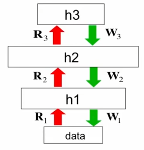
1. Backward (wake) phase: compute posterior using the recognition weights R. We assume independence.

2. Forward (sleep) phase: assuming correctness of posterior, learn the generative weights W by using MLE (because you already have the hidden states and the data). Just try to generate h2 from h3, and so on and so forth.

This is the genesis of the EM algorithm and various other algorithms. A forward backward process.

Problems

Mode averaging: because you assume independence, you may not be able to get the right distribution. You create a mode averaging situation where you are very wrong because you tried to interpolate between two rights

A good example is to think of learning the recognition weights for the V structure, where you’ll see that it’s wrong.

More information

https://www.youtube.com/watch?v=evnofrn-QHo&ab_channel=ColinReckons

Stacking RBMs

So we can combine the wake-sleep algorithm with retricted boltzman machines. You might have an RBM deep in a model that generates things based on MCMC, and then you use wake-sleep for the rest of the propagation

And at this point, we have moved ourself close to neural networks. The is more theory, but it’s not necessary to learn at this time