Natural Gradient

Tags	Second Order

Natural Gradient

What is gradient descent?

Gradient descent is actually technically a solution to the constrained optimization problem: $\min f(x)$ such that $||x’ - x|| < \epsilon$ . By the nature of the descent algorithm, the metric is usually L2 distance (because you take a set step in the direction of the gradient. If you write out the Lagrangian and solve, you get the traditioanl gradient update

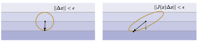
\theta' \leftarrow \theta -\alpha \nabla f

However, this assumes that all steps in parameter space are equivalent in objective space. Unfortunately, this is a very strong assumption. What if the loss terrain is oval-looking?

Steepest descent update

Here’s the insight: if we can estimate the second-order curvature of the terrain, then we can compute the step of steepest descent. In normal gradient descent, we assume that the hessian $H = I$ . This is apparent when you write the constraint in terms of a quadratic form

||\theta' - \theta||^2 = (\theta'-\theta)^TI(\theta'-\theta)

But this opens up the opportunity for a more general metric $||\theta’ - \theta||_H$ . These metric sare known as Mahalanobis metrics

||\theta' - \theta||_H = (\theta'-\theta)^TH(\theta'-\theta)

Now, if we plug this constraint into the Lagrangian, you get this new update rule:

\theta'\leftarrow \theta - \alpha H^{-1}\nabla_\theta f

Connection to Newton’s Method

So this is very similar to Newton’s method. In fact, it’s identical to the damped Newton’s method. But philosophically, we care about this because it shows us how we can modify our gradient to maximize the descent. It still is, at heart, a first order method.

Fisher Metric

A common application of the natural gradient is when you want to do the following optimization: you want to $\max_\theta f$ such that $D_{KL}(p_\theta || p_{\theta’}) < \epsilon$ . A good example is in policy updates, where you want to keep the new policy as close as possible to the old one.

Here, we use the critical insight that the second-order Taylor approximation to KL divergence is the Fisher Information Matrix.

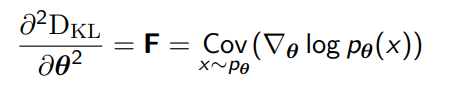
which can also be rewritten as

F= E[(\nabla \log p_\theta) (\nabla \log p_\theta ^T)]

and so the update is

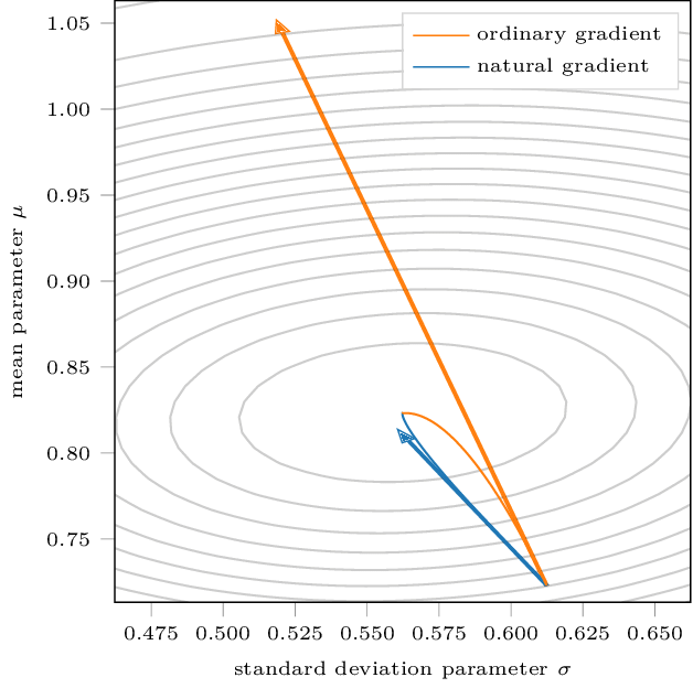
\theta'\leftarrow \theta - \alpha F^{-1}\nabla_\theta f

Because we care about distribution space, the updates with the Fisher Metric are invariant to parameterization.

Simplifying the Natural Gradient

☝

For more details, see http://arxiv.org/abs/1503.05671

The problem is inverting this Fisher matrix. Researchers are able to simplify the calculation by making some simplifications

Assuming that activations and gradient are independent. This creates an elegant decomposition of the Fisher matrix into Kronecker products

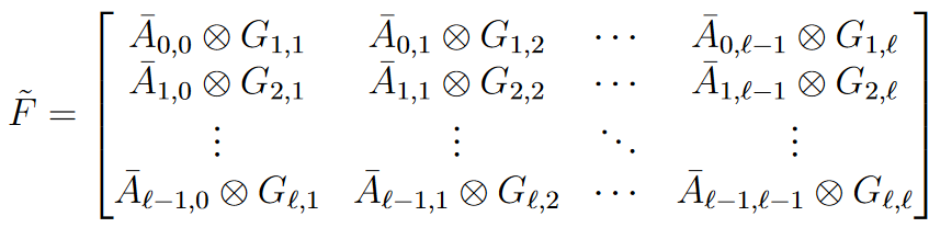
This allows the fisher matrix to be approximated as a Block-diagonal inverse by using Kronecker identities

This also allows the fisher matrix to be approximated as a tri-diagonal inverse by using some more complicated inference techniques

There are some really elegant connections to PGMs and other fields.

Most critically, the simplicity of the inverse doesn’t mean simplicity of the normal matrix, which means that the approximations are not too strong.