The idea

Ok, the jacobian tells us about the derivative of a $m → n$ function. What about the second derivatives of a $n → 1$ function?

You can imagine constructing the hessian as follows:

So essentially the row and column correspond to the first and second derivative, respectively.

Properties of the Hessian

Because of the Clairaut theorem, $\frac{\partial^2}{\partial x_i \partial x_j}f(x) = \frac{\partial^2}{\partial x_j \partial x_i}f(x)$. As such, $H$ is symmetric!

From this, we know that it has an orthogonal basis of eigenvalues. Furthermore, we know that the directional second derivative is $d^T H d$, where $d$ is a unit vector. It can be interpreted as weighted sum of eigenvalues (just split $d$ into a basis of eigenvectors and you will see why).

Alternative understanding of $d^THd$

You can also see $H$ as a matrix representation of a quadratic form, where the diagonals represent a scaled version of $x^2, y^2, ...$ and the non-diagonals represent stuff like $xy, yz, xz$. You can understand this like a quadratic form because $H$ is essentially estimating the function $f$ as a quadratic form!

Intuition of the Hessian

The hessian gives a sense of "curvature" of the function. The first derivative is the slope, and the second derivative is how that slope changes. This is particularly useful, because sometimes when you're optimizing a function, going the steepest way down is NOT the best thing to do. More on this later.

Second derivative test with the Hessian

The second derivative test is possible with the Hessian through eigendecomposition. To be more specific, we look at the eigenvalues of $H$. If they are all positive, then it is positive definite and we are in a local minimum. The intuition is that all the directions yield a positive curvature, which means that we are sitting in a divot.

If they are all negative, then it is negative definite and we are in a local maximum. If there are zeros, then we are undefined. The intuition is that in some directions the curvature is zero, which doesn't tell us much. Graphically, it may look like a taco shell, or it can be really weird (see below)

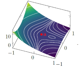
If you have both positive and negative eigenvalues, then you are in a saddle point. Intuitively, this means that going some directions you will have negative curvature and going other directions you will have positive curvature.

Hessians and learning rate

Instead of approximating the slope at one point, why don't we approximate the curvature in the form of a quadratic form? Perhaps we can gain more insight at how the gradient descent performs

The math

More specifically, we do a second-order Taylor series approximation to get this:

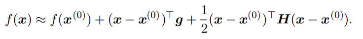
The $g$ is the gradient. The first component is the value, the second component is the directional derivative, and the third component is the second directional derivative.

If our learning rate is $\epsilon$, then our step is represented as $x^{(0)} - \epsilon g$. If we plug this in as $x$, we get the following

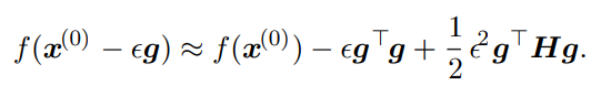
As such, our performance depends on this $\epsilon^2 g^THg$ term, or in other words, the square of the learning rate times the directional derivative in the direction of travel. If the last term is too large, we can move uphill (this formalizes some of the intuitions we had of gradient descent. If this term is zero or negative, then the formula predicts that we can get infinite improvement with an infinite learning rate. This isn't really true, because quadratic appproximations are local only.

However, with this formula we can find the $\epsilon$ that decreases $f(x^{(0)})$ the most, by a simple quadratic minimization. This gets us

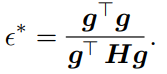
What's the implication? Well, if $g$ aligns with the largest eigenvalue, then $\epsilon^* = 1/\lambda_{max}$. Anything less, and $\epsilon^*$ will be larger. As such, it is best to upper-bound your $\epsilon^*$ WRT the largest eigenvalue of the hessian.

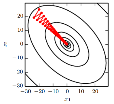
Condition number of the hessian

This, again, is the ratio of the largest and smallest eigenvalues. Now, this kinda tells us how "lopsided" the local topology is. Gradient descent performs poorly with a bad condition number. why? Well, it means that the loss is super sensitive to which direction you travel. As such, you must use a small learning rate, and you might bounce around a lot