The idea

What if we wanted to find the maximum or minimum of a function GIVEN that you must stay within some bounds? For example, "what is the highest point on the US interstate system?"

The intuition

Every non-extreme value must occur at least twice on a constraint surface. "what goes up must come down". However, the extreme values may occur only once! Intuitively, this means that the contour "kisses" the constraint edge without penetrating it.

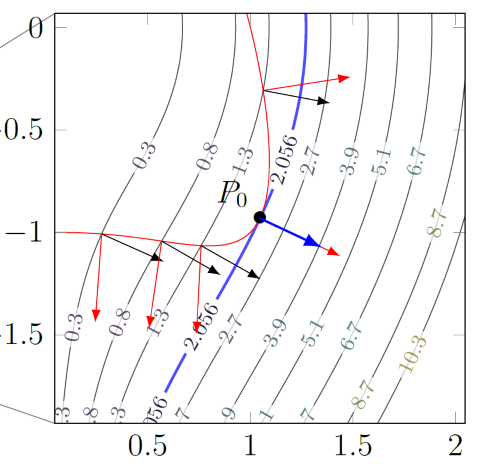
Let $f(X)$ be the function we want to optimize, and let $g(X) = c$ be the constraint. Note how $g(X) = c$ is just a contour. If we took the gradient $\nabla g(X)$, the gradient would be orthogonal to the contour. As such, the constrained optimum can be represented by the following equation:

Intuitively, when a contour $f(X) = k$ kisses $g(X) = c$, the gradients are colinear.

Solving for these points

In $\mathbb{R}^n$, the $\nabla f = \lambda \nabla g$ gives us $n$ equations. However, we need $n + 1$ equations because we introduced the $\lambda$. This is where the $g(X) = c$ comes in, with the last of the equations!

The mechanics of solving:

• solve for $\lambda$ in as many expressions as possible, then set them equal

• if you divide by a variable, you must produce cases where that variable is zero and non-zero

• If $\nabla g$ vanishes, you must also consider that as a candidate point, as long as that is on the curve

If you're on a closed curve, then you will have two local extrema. If you are on an open curve, you can have neither.

The legrangian

The legrangian is defined as

(this can be expanded for more than two variables). The solution to the constrained optimization is when $\nabla L = 0$. This is not a new technique; it's just a way of packaging what we saw before into one clean equation.

Intuition of the legrangian

This really begs the question, as the legrangian seems to be able to transform constrained optimization into universal optimization. You can think of $L$ as being the function $f$ with a "penalty" component. Everywhere on the constraint, you are simply optimizing $f$. Everywhere outside the constraint, you are either adding something or subtracting something. This "something" will prevent the legrangian from having a zero gradient, which is shown algebraically.

As an aside, you see that $\frac{\partial L}{\partial c} = \lambda$. Now, when we are on the constraint, $L = f$. As such, we can understand $\lambda$ to represent how the extreme values change WRT the constraint! In other words:

where $M_f$ is the extreme values.

Another intuition of the Legrangian

You can also think of optimizing the legrangian as doing this (or with $\min$)

If the constraint $g(x, y) = c$ is not satisfied, then the max would cause the whole thing to go to infinity. As such, to optimize the Legrangian is to perform constrained optimization

Multiple equality constraints

If you want to optimize a function subject to two constraints, it turns out that the gradient must lie in the SPAN of the constraint contour gradients.

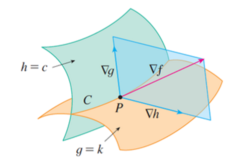
As such, $\nabla f = \lambda \nabla g + \mu \nabla h$. We can solve this in the exact same way as before!

Karush-Kuhn-Tucker

Here, we do something a bit harder and a bit more practical. What if we wanted to optimize a function $f$ subject to the constraints $g_i(x) = 0$ and $h_i(x) \leq 0$??

Generalized Legrangian

We create the generalized legrangian as follows:

such that $\mu \geq 0$.

Using the Legrangian

Now, let's attempt to find the extrema:

If $g(x) \neq 0$, then the $\lambda$ optimization will go to infinity. If $h > 0$, then the same thing will happen during $\mu$ optimization (currently, $\mu h$ is negative so maximizing is constrained)