Constrained optimization

Consider the following problem:

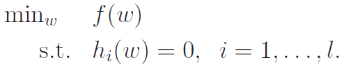
You can use the legrange multiplier method to solve this. As a shorthand, we can also use the Lagrangian, which is expressed below

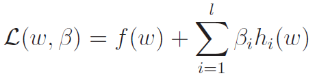
This is convenient, because the Lagrangian maps the constrained optimization problem into an unconstrained optimization problem. The critical points where $\nabla \mathcal{L} = 0$ are your critical points on the original constrained optimization problem.

This is super helpful for simple constraint problems. But now we will concern ourselves with optimization problems with constraints, which can be more common.

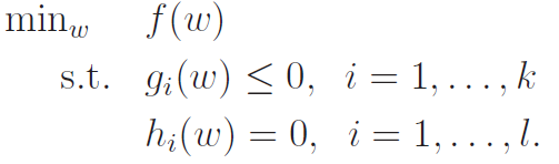
Generalized Lagrangian

In addition to equality, the generalized optimization problem has inequalities as well. We call these primal optimization problems.

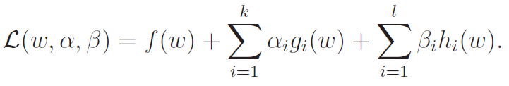
We define the generalized Lagrangian below:

Now, how the heck are we going to use this? Well, we could consider defining a maximization problem as below

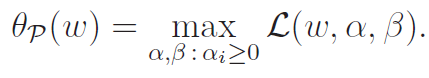
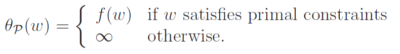
(the $p$ stands for primal.) Now, let's understand why this makes sense. If $g_i > 0$, we see that $\theta_p = \infty$. this is because you could make the $\alpha_i$ arbitrarily large. If $h \neq 0$, then the same thing happens. We can make the $\beta$ arbitrarily positive or negative to make it infinity. It is only when these conditions are satisfied that $\theta_p$ is finite.

As such, we can reframe our objective as a min-max problem

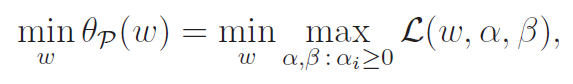
We define $p^* = \min_w \theta_p(w)$, and when we find that minimum, we can obtain the argument $w$ that minimized $\theta_p$

Legrangian Duals

Now, we are going to dive a little deeper on min-max vs max-min. We propose a dual $\theta_D$ as defined as follows:

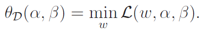
The dual optimiazation problem is thus

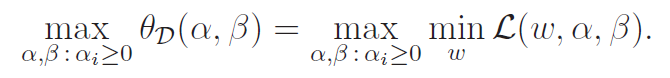
Now, what is the difference between max-min and min-max? The maximum of the minimums is smaller than the minimums of the maximums. This the idea that the highest chair on the floor is still shorter than the lowest bump on the ceiling. As such, we get

Necessary dual conditions

There are some conditions in which $d^* = p^*$, which allows us to solve the dual problem instead of the original problem. This is beneficial because the min is unconstrained, while the max is constrained. It might be easier to do unconstrained optimization first.

First, we suppose that $f, g$ are convex (hessian positive semidefinite) and that $h$ is affine (linear with intercept). With these exceptions only, we can say that $p^* = d^*$!! Nice!

Interestingly, under these conditions, we get that $w^*, \alpha^*, \beta^*$ satisfy the Karush-Kuhn-Tucker (KKT) conditions:

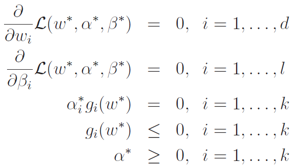
Specifically, we care about $\alpha g_i(w) = 0$ This we call the KTT Dual Coomplementarity condition. This shows that in optimality, if $\alpha$ is non-zero, then $g_i(w) = 0$, meaning that it is at its limit. We call this constraint as being active, as we have turned the inequality $g(w)\leq 0$ into an equality.