Flavors of recurrent neural networks

• one to many: image captioning

• many to one: action prediction

• many to many with intermediate representation: video captioning

• many to many (direct 1:1 correspondence): video classification on frame level

Other uses of sequential processing

You can use a sequential processing approaches to take “glimpses” of an image to classify it. This models how we take in information. We can even use a sequential model to generate things!

Various applications

• image captioning: encode the image and then take this embedding and generate text from a one-to-many RNN

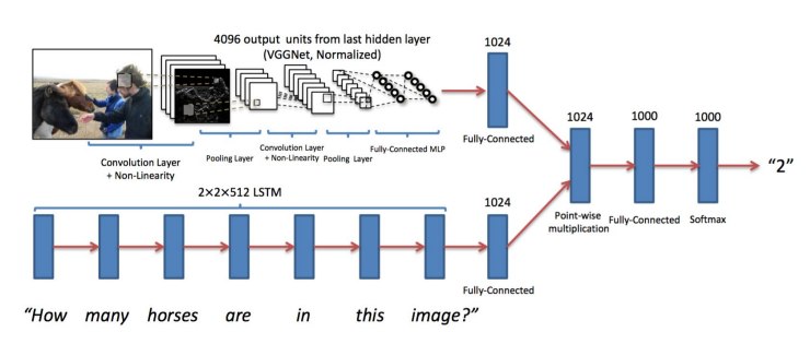
• visual question answering: encode the image and the question, and this work attempts touring them

The structure

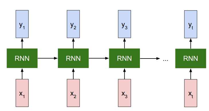
The RNN has an intermediate representation that is kept through time. It acts like “memory.” The functional definition is actually pretty simple

And then you define

This we call the Vanilla RNN. Now, the $y_t$ may not necessairly be our output; it can be an intermediate represention that we decode later. You can have multiple hidden layers like this

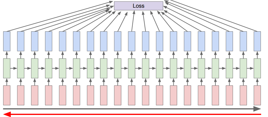
Many to many

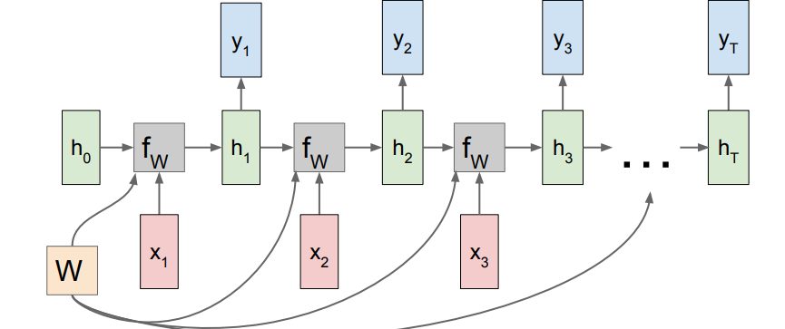
This should be pretty self-explanatory. You add the losses together at the end

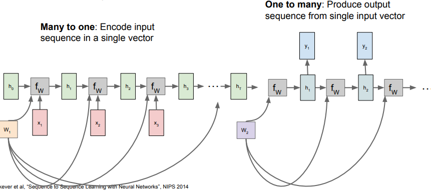
Many to One

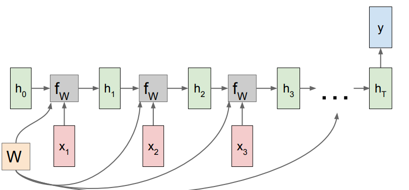
This just takes the final hidden layer and uses it for the prediction. Other models might average the last $k$ hidden layers for more stability.

One to Many

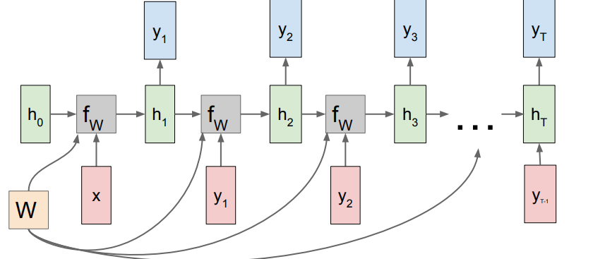
We just feed in the single $x$, but to be mathematically legal, we “backfeed” the last output as the next input, because the shared weights expects an input.

Many to One + One to Many

If you’re doing someting like video captioning, you would want to extract the “essence” of a video and then write a caption on it. This yields the two different architectures chained together

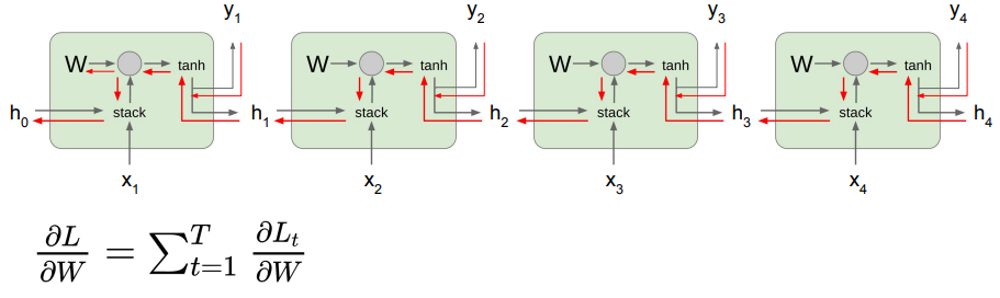
Backpropagation

Backpropagating an RNN is actually not very fun. You basically have to roll out the network through time, as the loss is influenced by each timestep

To be more specific, for every hidden layer before you propagate to $dW$, you have the $dH$ from the loss, but you also have another $dH$ from the next hidden layer. You add these together to backpropagate to $dW$ and $dX$

Truncated backpropagation

For a feasible backprop algorithm, we just slide a window across the sequence and do full backprop this way. However, at the end, we slide the window over to the next chunk. We keep the hidden representation we got from the last chunk, and we also change the weights of the LSTM to reflect the updates made in the last sliding (to be more efficient)

LSTM

What’s wrong with RNNs?

The tl;dr is that we compute repeated products to compute $dL/dh$, which yields either an exploding or a vanishing gradient

• Details

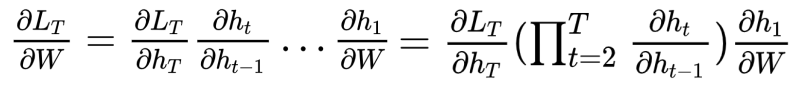
  To compute the derivative, we sum the contributions at each time set

  

  This involves a repeated composition of the $\frac{\partial h_t}{\partial h_{t-1}}$ term. From this, we can express the gradient as

  

  What’s wrong with this? Well, let’s look closer. We can express the hidden propagation using block notation:

  

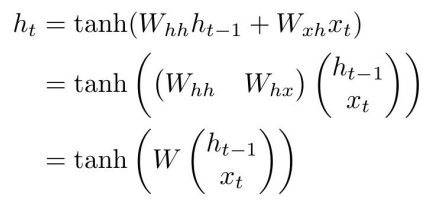
  And we compose this function over and over to get the subsequent hidden layer. If we compute the derivative, we get

  

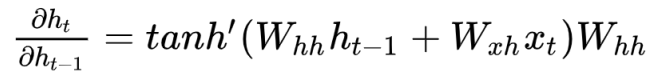
  and we should see a problem immediately. The hyperbolic tangent function is a crushing function, meaning that repeated composition will push earlier $x_t$ contributions to zero. This isn’t good, as it imposes a set of blinders on the RNN. We call this the vanishing gradient effect.

  We might try to fix this by removing the $\tanh$ activatino, but we still are in a precarious position. We are raising $W_{hh}$ to a power $T$. If the largest eigenvalue of $W_{hh}$ is less than 1, then we get vanishing gradients, and if it’s greater than 1, we get exploding gradients. So it’s too sensitive. Can we do better?

A typical RNN is able to look around 7 timesteps back.

The LSTM formulation (intuition)

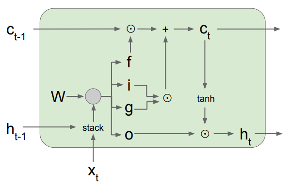
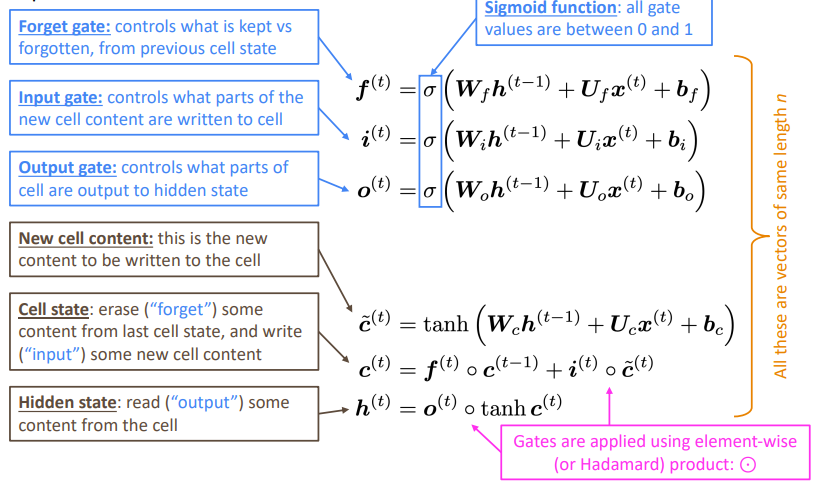
In the LSTM there is a cell state and a hidden state. The hidden state is derived from the cell state. The hidden state is used as context in determining the other gates. Note how the cell state is not used in the weight multiplication.

The forget gate decides how much of the past cell state we should remove. The input gate decides how much of the past cell state we need to change. The gate gate (stupid name) suggests changes to the cell state. And again, finally, the output gate decides how much of the cell state is relevant for the next round of gate determining.

The LSTM formulation (practicals)

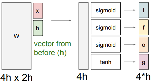
Using block notation and a slight abuse of notation in activation function, we define the LSTM to be

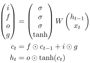
Basically, from the input and the last hidden layer, we create a set of outputs. This is a good diagram of how this happens

The gradient superhighway

The key insight of the LSTM is that the memory branch is only modified by element-wise operations, which are very easy to backpropagate through. Furthermore, if we wanted to keep the cell state as-is, we just need to set $f = 1, i = 0$. In contrast, it would be very hard to keep $h_t = h_{t-1}$ in an RNN because there’s a matrix multiplication in the way.

The derivative of $W$ depends only on $c_{t-1}$ at each point, so if $\frac{dL}{dc_{t-1}}$doesn’t become small, then the derivative WRT $W$ at each timestep also doesn’t become small. Nice!!

In a way, we can understand the cell state as a sort of residual connection.

Caveats

The LSTM makes it possible to not have the vanishing or exploding gradient, but it doesn’t guarantee it; it just makes it easier.

Other variants

The GRU (Gated Recurrent Unit) is also popular.

Other ways of dealing with exploding/vanishing gradient

So for exploding gradient, we can just clip the gradient and things usually work pretty well.

For vanishing gradient, we can use residual connections between the layers, like what Resnet does. We can also add dense connections, which connect each layer to all its downstream layers. This works for feedforward networks.

We can also apply a more gated connection to these networks, and we stumble upon essentially the LSTM version of a feedfoward network.

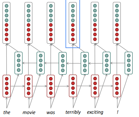
Bidirectional and multilayer models

We can consider adding more complexity to the LSTM. First, we can add another layer that looks backwards. This critical because now, each word has both forward and backward context

You can also add more layers to an RNN, and this functions like layers of a CNN. Each successive layer pools more information across time, which yields higher-level features.