GUEST LECTURE BY HANIE SEDGHI

What is being transferred in transfer learning?

Low-level statistics

• Common belief: transfer learning benefits come from feature hierarchy learned during pretraining

• However, if you shuffle the downstream task image features (i.e. literally cut up the image and reposition it), you still get a benefit over random initialization

• this indicates that there are other factors at play, like lower-level statistics about the data (image color histograms, etc). The speed of optimization is especially boosted

Shared optimization basin

If you take two model parameters of a network and linearly interpolate between them, it is likely that you will see a “valley” where the in-between parameters are no better than random guessing. This makes sense, as the parameters are highly non-linear.

You can interpret this result as the networks residing in two separate loss basins, which means that you must walk over a hump to get to the next one.

• Two networks initialized randomly and trained on the same data will still be in separate basins, if the ordering of data is different

However (and this is the cool part) two models fine-tuned from the same model will be linearly interpolable.

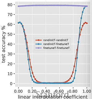
In other words, these models lie in the same basin, which means that you can actually use any models from the interpolation, resulting in an easy ensemble!

Which layers are more important?

You can generate a plot where you take a layer and linearly interpolate between its starting distribution and its ending distribution. You add noise and plot how sensitive the model is to noise at different points of interpolation.

As we move from the input to the output of a network, the criticality of the weights tend to increase (i.e. the viable parameter “ball” around the true parameter becomes smaller.

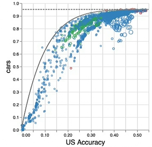
The limits of large-scale pretraining

Effect of scale

People tend to think that with more data and larger models, we get non-saturating performance. This does seem initially true; pretraining and downstream accuracies tend to be linearly correlated

In reality, if we do a much wider sweep (across many types of models, data, etc), we get something that looks like a logarithmic curve