Reconstruction methods

The big idea is that we want to train a representation by somehow using a reconstruction objective, like an autoencoder.

Autoencoders

An autoencoder essentially forces a compression of an input into a representation space, and then decompresses it to match the original input as much as possible.

Then, during few-shot learning, we can strap a head onto the encoder output and train that lightweight head directly

The problem is that we need to make an information bottleneck, and it’s not trivial to provide a good bottleneck. If the task isn’t hard enough, you might end up with essentially a hash function that doesn’t do a good job at representing the critical features.

In general, autoencoders yield poor few-shot performance.

Masked autoencoders

One problem is that the task of an autoencoder is too easy. Essentially, construct $x$ from $x$. Instead, we might feed in one part of an input and ask the autoencoder to reconstruct the other part. You would feed in one part of the input and ask the model to infer what was under the mask.

For images, you can just add a visual mask, and for text, we will use a mask token (more on both later)

BERT as a masked autoencoder

The big idea is that BERT can take in a sentence and output a distribution for every token after being run through attention. So, this is sort of like an autoencoder, and you can feed in a <mask> token and see what the BERT model outputs at the other end. It’s going to be a distribution, and you minimize the KL divergence between this distribution and the one-hot distribution of the true word

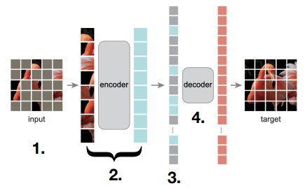
Masked visual autoencoders

A very similar idea: remove parts of an image and try to reconstruct the whole image

Which do I use?

Masked autoencoder paradigms tend to do better when fine-tuned (because they capture more information), but contrastive methods tend to yield better out-of-box (linear probing) accuracy.

Transformers review

A transformer basically takes in a set of embeddings and in each transformer block, uses a multi-head attention block to “stir up” the embeddings. Otherwise, the embeddings are kept separate.

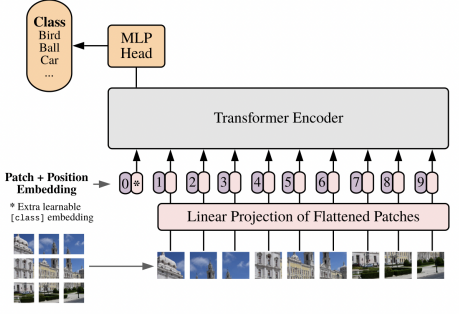
If you want to yield a prediction, you feed in a zeroth token, and you extract the embedding from that token after the transformer to yield the prediction. This is OK, because eventually the transformer will learn to pull information from all embeddings to this point.

The transformer block

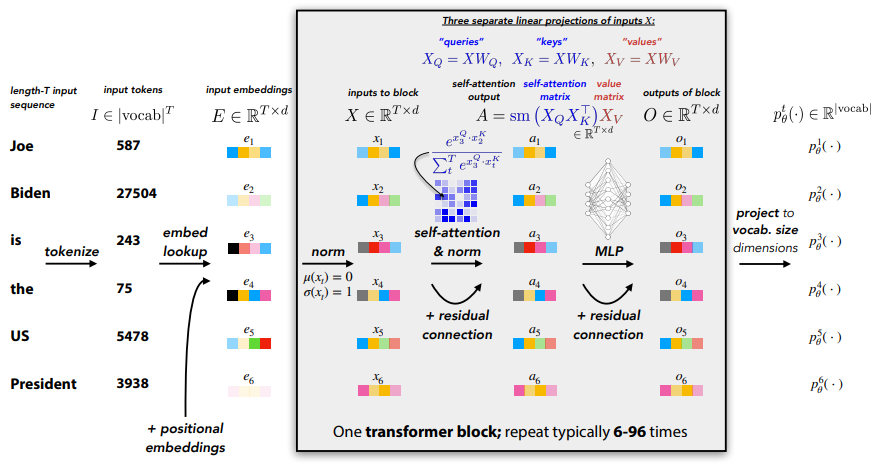
We feed in embeddings into the transformer. This can come from an image encoder, or it can come from an embedding lookup for text. Then, we perform self-attention.

Self-attention essentially yield a matrix $A$ whose $A_{ij}$ is how similar embedding $i$ is to embedding $j$. This is computed through a batched matrix multiplication that computes pairwise inner products. Now, when you multiply $AX_V$, you’re keeping the embedding dimensions independent, but you’re mixing the different embeddings according to each row of $A$ (you’re actually computing a convex sum due to the softmax). This is in contrast to computing $X_V = XW_V, X_k, X_q$, where you’re keeping the embeddings independent but mixing together the embedding dimensions.

The big idea is that self-attention allows you to “select” a combination of embeddings directly, which allows you to pay attention to things long ago in the past. While the $X_QX_K^T$ procedure feels very brute force, do know that you can learn $W_Q, W_k$, which means that you have control over what the $X_QX_K^T$ outputs, and therefore control over what to attend to.

Again, note that all of the embeddings are independent except when you do self-attention.

In the real implementation, they use a 1d convolution across the sequence of embeddings with kernel size 1, which is equivalent to doing the MLP for each embedding and concatenating.

Fine-tuning transformers

You can take the representation of that [CLS] embedding (the first thing we feed and what we choose to extract) and apply a prediction head. This can work, but what do you do with the transformer?

You can try to fine tune the model “a little bit.” To help with intuition, consider the matrix product $Wx$. We can rewrite it as

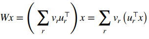
or a linear combination of “memories” stored in $W$. As the $v_ru_r$ is created through SVD, where $u$ is orthogonal and the $r$ stands for a sum over ranks, each “memory” is just one rank. We know that some $AB^T$, $A, B \in d \times p$ is a low-rank matrix (where $d$ is the size of the main matrix $W$). So, we can constrain the update to

This is LoRA approach! We make low-rank changes to weights

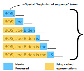
Autoregressive models

This is actually the same as a masked model except that you mask in a regularized way. You always make the last element you feed in the mask, so you’re essentially aking the model to fill in the next word.

To be clear, when you feed in a transformer, you input a sequence of length $n$. The transformer also outputs a sequence of length $n$. The $k$th element of the output is the prediction of the $k + 1$th token.

Then, during training, you will put the right answer (even if the model was wrong) and train the next word. The big advantage is that you can do all these masking predictions in one run, while the previous masked models, you would need to rerun the whole model when you tried a new mask.

The downside is that you force the model to only look backwards. Sometimes, when you’re trying to understand a sequence, it can help to look forward as well.

Contrastive learning vs AEs vs Masked AEs

Contrastive learning yields high quality representations with a small model, but the negative selection is tricky, and generally needs larger batch size

Autoencoders are easy to implement but you need a larger model and requires a special bottleneck with relatively poor few-shot performance.

Masked autoencoders are better few-shot performers and can give a generative model if you use an autoregressive setup. However, without fine-tuning, the raw representations may not be good.