Optimization-Based Meta-Learning

Tags	CS 330Meta-Learning Methods

Moving to optimization

In black-box approaches, we outputted parameters $\phi_i$ as a function of the training set $\phi_i = f_\theta(D^{tr})$ . (or we did it implicitly through an RNN).

However, what we really want is some sort of “quick learning” that yields $\phi_i$ , and during learning, we use gradient descent. Can we put this inductive bias into the function $f_\theta$ ?

As it turns out, yes!

Optimization-based adaptation

We can just define

\phi_i \leftarrow \theta - \alpha \nabla_\theta \mathcal{L}(\theta, D^{tr})

with a meta-objective being

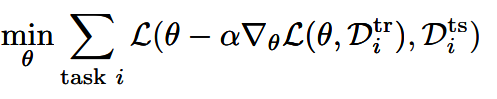
So this is essentially like fine-tuning, but we are optimizing for the ability to be fine-tuned. This is known as Model-Agnostic Meta-Learning, or MAML.

the $\alpha$ is typically larger than the standard learning rate, and there may be more than one gradient step. We will talk about this in a second, during the math theory part.

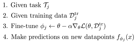
The algorithm

The math theory

But this raises some big questions. We are taking a gradient through an optimization procedure. Does that mean we need to take the hessian?

Actually, no! As it turns out, we can express hessian-vector products without actually computing the hessian. We will explain why we care about this in a second.

If we let $g = \nabla f$ , then we have the first-order taylor expansion $g(x + \Delta x) \approx g(x) + H(x)\Delta x$ . Now, we can express $\Delta x = rv$ , where $v$ is a unit vector and $r$ is a scale. This means that $g(x + rv) \approx g(x) + rH(x)v$

This means that you can solve for $H(x)v$ .

H(x)v \approx \frac{g(x + rv) - g(x)}{r}

which means that you only need two points of the gradient to approximate the hessian vector.

All of this is cool, but why do we care? Well, let’s crunch the numbers and compute the gradient of the meta-objective

\nabla_\theta L = \nabla_\phi L(\phi, D^{ts})|_{\phi = \phi_i} * \frac{\partial \phi_i}{\partial \theta}

And of course, because $\phi_i$ relates to $\theta$ through the derivative, you will need the hessian.

\frac{\partial \phi_i}{\partial \theta} = I - \alpha H(x)

Now, this nasty $\nabla_\phi L(\phi, D^{ts})|_{\phi = \phi_i}$ is a computable row vector that we can call $v$ . Therefore,

\nabla_\theta L = v I- \alpha vH(x) \approx vI - \alpha \frac{\nabla_\theta(x + rv) - \nabla_\theta(x)}{r}

where $r$ is a small number.

as it turns out, Pytorch does all this heavy lifting for you, so you dont’ have to worry. But it’s always important to know where things come from.

If you take more than one gradient step, you can actually show that it doesn’t increase the order of the derivative. Intuitively, you’re applying a first derivative over and over, but you’re not differentiating with respect to it. So, while the expression becomes more complicated, the order stays at 2.

As a proof sketch, you can show it inductively. $\phi_i \leftarrow \theta’ - \alpha \nabla_{\theta'}L$ , and it yields the same form but you multiply the end by $d\theta’ / d\theta$ . Now, you can write $\theta’ \leftarrow \theta’’ - \nabla_{\theta’’}L$ and you get the same form, but you need $d\theta’’ / \theta$ . (note that the primes are not derivative but just updates.). You keep on going until you get to the original $\theta$ . So you can imagine rolling out the derivatives in reverse.

Now, due to the chain rule, all you’re doing is taking products of hessians. You are never taking a deeper gradient.

Optimization vs black-box

MAML is like black-box, but the computation graph has a gradient operator. You can also mix-and-match, where you might have a function $f$ that takes in $\nabla_\theta L$ and modifies it to form the gradient update for $\theta$ .

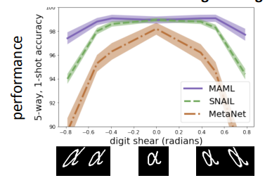
In general, because we know that optimization does something reasonable (moves us towards lower loss), it has better behavior with out of distribution or extrapolation examples. We can also show that MAML is expressive as any other network along with the power of this inductive bias of learning.

Pros and cons

One challenge is that bi-level optimization is unstable at times. Here are some solutions

learn the $\alpha$ along with the $\theta$

optimize only a subset of parameters

introduce context variables

Another challenge is that the inner gradient step is heavy on memory and compute

Crudely approximate $d\phi_i / d\theta = I$ , which actually kinda works for simpler problems, as this assumes that the optimization terrains stay roughly the same.

Optimize only the last layer of weights (can yield convex objective)

Derive meta-gradient using implicit function theorem (see paper Implicit MAML)

So the big takeaways is that there is a good inductive bias, better extrapolation, and model-agonistic. The cons is that it’s more memory/compute intensive and requires second-order optimization.