What is unsupervised pretraining?

This is what happens when you have a diverse unlabeled dataset, and you want to pretrain a model such that it is easy to fine-tune for a desired task, using a small number of labeled training data?

Contrastive learning idea

The big idea is to create an embedding space that pushes similar things together and different things apart.

Constructive positive examples

There can be many approaches to this. If you have access to class labels, just draw from the same class. If you end up doing this, your approach becomes adjacent to Siamese nets and ProtoNets.

You can also use nearby image patches, augmentations, or nearby video frames.

Constructing negative examples

You can’t just push similar examples closer to each other, because there exists a degenerate solution that just outputs the same embedding for any input. You need to compare and contrast.

Triplet loss

One such way of making negative examples is to pick three examples: one anchor, one positive, and one negative example. You want to compute

You use a hinge loss because the second term is unbounded, and you don’t want to have an exploding embedding space.

There are quite a few challenges of triplet loss. The main one is finding a good negative example. One negative example might not be enough.

You can interpret the triplet loss as the Siamese paradigm but you chop off the head and train a metric space instead of a classifier. You can easily derive a siamese network from a trained $f_\theta$ by making the last layer a sigmoid.

N-pair loss objective, SimCLR

This is just an extension of the triplet loss, where you want to separate one positive example from all the negative examples. This looks like

As a side note, we don’t add the positive example in the denominator, so it is slightly different than a simple softmax. The intuition is that you just want relative distance to negatives.

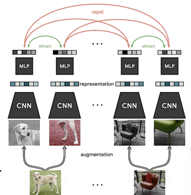
In the SimCLR algorithm, we generate positive pairs through augmentations from the same image and negative pairs between different images.

And the n-way loss is just all same-image embeddings divided by different image embeddings

Jensen’s inequality and Batch Size

As it turns out, these ways of contrastive learning requires a very large batch size. There’s actually a mathematical explanation.

Note how we are taking the sum of logs. In standard sub-sampling, you might have $\sum_n L(\theta, x^{(n)})$ and the loss is linearly composable. In other words, it makes no difference if you sum the loss (minibatches), or you optimize all at once (whole batch). The variance changes, but sums are interchangable.

However, now we are dealing with a log of sums (the denominator). If we do minibatches, it’s almost like we pull the sum out of the log and do partial sums. Jensen’s inequality tells us that

which means that for non-whole batch sizes, you are optimizing a lower bound of the loss objective. This gives you weak guarentees (ideally, you want to optimize an upper bound of a loss objective).

Solutions to this problem

• store representations from previous batches (MOCO)

• predict representations of the same image under different augmentations, which is sort of a bootstrapping operation. It doesn’t require negative samples. (BYOL)

• You can also go beyond augmentations
  • learn augmentations adversarially (Viewmaker Networks)
  • learn time-contrastive representations on videos (R3M, contrastive RL)

• image-text contrastive pretraining (CLIP)

Pros and cons

Pros

• good general framework

• no generative model

• can use domain-specific knowledge through types of augmentations and positive/negative examples

Challenges

• hard to select negative exaples

• requires large batch size due to Jensen’s inequality

• hard to get better performance than augmentation strategies

Contrastive learning as Meta-Learning

You can imagine setting up contrastive learning as a meta-learning problem.

1. Take an unlabeled dataset

2. Each datapoint in the subsample becomes a label class, and you create a data augmentation on each datapoint. Every sample from this original datapoint corresponds to the original class.
   1. so if you have a batch size $N$, this is your $N$-way classification
   2. You augment the data $K$ times, which corresponds to your $K$ shot.

There are a few differences though. SimCLR samples one task, but metalearning usually samples multiple tasks. SimCLR also compares all pairs, while metalearning compares queries from the same task.

However, if you frame this as a prototype network paradigm, you get some neat mathematical similarity.