Uncertainty

Meta-learning inner loops are expressive and are consistent with our current approaches, but they dont express epistemic uncertainty very well.

Version 0: Output distribution over predictions

If you fit a function to output a distribution over the predictions, like categorical, gaussians, or mixture of gaussians, this could work to express aleatoric uncertainty. It is also simple and can be combined with many methods. You would train by doing MLE to the target label.

However, you can’t reason about uncertainty over the underlying function (epistemic uncertainty) and it’s hard to represent an arbitrary distribution over the y-categories. And in general, the uncertainty estimates are poorly calibrated. Neural networks tend to be more certain than they should be.

What we really want is a model that outputs $\phi$, the learned parameters, as a distribution. If we could do this, then we would have accounted for epistemic uncertainty.

Variational Black Box Meta Learning

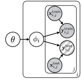
Why don’t we make a variational autoencoder with a slight twist. The input is the training data $D^{tr}$, the latent space is the parameter space $\phi_i$, and the output reconstruction loss is the test set $D^{ts}$. Let’s unpack this for a second.

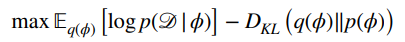
We want to optimize this following objective

Encoder $q$

What should $q$ condition on? Remember that from variational inference, this $q$ could be anything. We choose to let it be conditioned on the training set. This is the encoder of the VAE

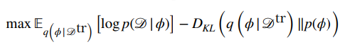
This actually is very intuitive. The model takes in a dataset and spits out a distribution over $\phi$, the model parameters. You can think of this as the inner loop optimization step.

Decoder $p$

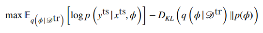
Now, a good “reconstruction” loss is to see how likely the test set is on the embeddings $\phi$. This is the decoder of the network, and it corresponds to a run through the generated model with parameters $\phi$

Using meta-parameters

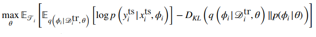
Where is the meta-parameters? Well, they are in $q$, and we often condition $p(\phi | \theta)$ on the meta-parameters, because the prior should be dependent on these meta-parameters.

Putting it together, we have…

Pros and Cons

The pro is that this represents any sort of distribution over $y^{ts}$ because you sample $\phi$ from a gaussian and then you sample the label based on some distribution like a gaussian. A composition of gaussians gives an infinite possibility of distributions when marginalized.

Another pro is that we actually have a distribution over functions now!

But the con is that our $\phi$ is still distributed according to a gaussian, so we don’t have as much expressive power.

Optimization Approaches

MAML as Hierarchical Bayes

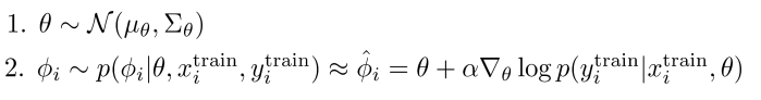
Given our dependency graph, our outer objective is

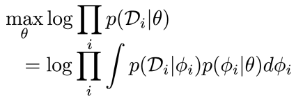
where this $p(\phi_i | \theta)$ is the inner loop parameter creation. In MAML, we just take the $\phi_i$ that maximizes this $p(\phi_i | \theta)$, which yields

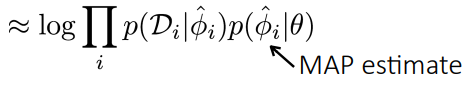
So we can understand gradient-based meta-learning as MAP inference! More on this in some papers.

The problem is that the framework is nice, but we can’t sample from $p(\phi | \theta)$, and that’s what we really want.

Bayesian optimization based meta-learning: MAML in Q

We can mitigate this by using the exact same structure we had before, but now we change this $q$ from a blackbox RNN to a computational graph that includes a gradient operator. You train neural network weights $\mu_\phi, \sigma_\phi$ on the training set (you would sample $\epsilon$ and use the reparameterization trick).

The problem is that this is still modeling $p(\phi | \theta)$ as a gaussian, and this is not necessailry the best choice. We are limited because of the reparamterization trick.

Bayesian optimization-based meta-learning: Hamiltonian Monte Carlo

The key goals is to sample from $\phi_i \sim p(\phi_i | D^{tr})$. We don’t know what the meta-parameters are, so we must marginalize.

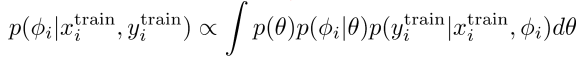
Now, if we observed this $\theta$, then we can easily just sample from $p(\phi | \theta, D^{tr})$, which we can approximate with the MAP in MAML we just talked about

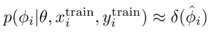
So we’re just doing ancestral sampling on the original PGM:

So we just do the following two steps to following the parent-child sample

Why do this? Well, intuitively, the model might have multiple different modes of optimality, and by sampling the metaparameters, we can get a better coverage.

The pro is that this has a non-gaussian posterior and is simple at test time. However, the training procedure is harder.

Ensemble Approaches

We can train an ensemble of MAML models. The distribution of models is a sample from $p(\phi | \theta)$, and there is no gaussian restriction. This works for black box, non-parameteric, anything!

The problem arises in getting models that are different. To solve this, we can add an additional loss term that pushes adapted parameters away from each other through a kernel similarity function

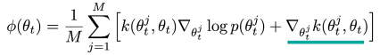
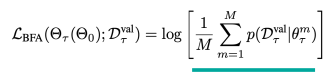
You optimize for a distribution of M particles that produce the highest log likelihood, so this is an MLE objective in a way.

The pro is that this is simple and very model agnostic, and it yields non-gaussians.

The con is that you need to maintain $M$ model instances!

Evaluating Bayesian meta-learner

You could use standard benchmarks, but the problem is that the tasks might not be ambiguous enough for these things to matter. You can use toy examples to help with diagnostics, like ambiguous regression or even rendering

You can use reliability diagrams, or you can plot active learning (i.e. as you pick the best data points for learning, how much better does it do as compared to random sampling?)