Ways of convergence, constraint

Asymptotic bounds: this guarantees that some $X → Y$ as $n→ \infty$ . You might get a high probability bound of $o(f(n))$, which gives a bit more structure asympotically

• Example: law of large numbers (loose)

• Pros: often the most intuitive, easy to work with

• Cons: may not say too much about low $n$

High probability bounds: this guarantees that $|X - Y| > \epsilon$ chance is $\delta$. you get an interplay between $\epsilon, \delta, n$. You can set two of them and the third one will be derived. Usually $\delta$ is written as a function of $n$, but you can easily invert

• Example: all tail bounds, hoeffding’s inequality

• Pros: strict definition, works on every $n$

General Tail Bounds

Tail bounds are important because they limit how large your tail is in a distribution, which naturally has implications for learning algorithms that could potentially exclude the tail of a distribution

Markov’s Inequality

This shows that the tail of a distribution is limited in size. Proof: write as integrals and you’ll see it.

Chebyshev’s Inequality

Now this is very interesting, because it shows that variance has something to do with convergence rates

General Tail Bound

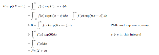
Claim: if $X$ is real, then for any $t\geq 0$,

• Proof (expansion into integrals)

  

Gaussian tail bound

Claim: if $Z$ is gaussian with mean 0 and variance 1, then

• Proof (general tail bound + moment generating function)

  

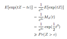
  and then let $t = c$, getting us

  

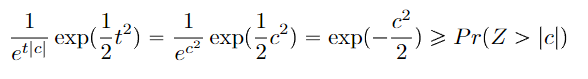
  If you want this to work with non-unitary variance, just plug in the non-unitary variance MGF of the gaussian and set $t = \frac{1}{\sigma^2}c$.

This gets us a stronger variant of Chebyshev’s inequality, and it is food for thought.

Hoeffding’s inequality

Hoeffding’s inequality in the general form is as follows: given $X_1, … X_n$ and $a_i < X_i < b_i$, we have

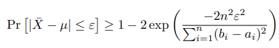
We often find a looser bound by replacing $b_i - a_i$ term with $\sigma^2$, because the range is always less than the variance.

Common forms include

• $2\exp(-2n\epsilon^2)$ if you are bounded in $[0, 1]$

• $2\exp(-2\epsilon^2/n)$ if you are bounded in [0,1] and you are dealing with SUMS, not averages.

• Proof (lots of algebra + Markov’s inequality)

  Start with $\bar{Z} = \sum(z_i - E[Z_i])$. If $\bar{Z} > t$, then $\exp(s\bar{Z}) \geq \exp(st)$ for every $s \geq 0$. Markov’s inequality therefore states that

  $$P(\bar{Z} > t) = P(e^{s\bar{Z}} \geq e^{st}) \leq \min_s\frac{E[e^{s\bar{z}}]}{e^{st}}$$

  After expanding back into $z_i$, you get that this is equal to $\prod E[e^{s(z_i - E[z_i]}]$.

  With Taylor expansion, you get that $E[e^{sz_i}] \leq e^s - s$. We know that $e^x - x \leq e^{x^2}$, which means that $\prod E[e^{sz_i}] \leq e^{ns^2}$.

  The minimizer of $\min_s\frac{E[e^{s\bar{z}}]}{e^{st}} = e^{ns^2}/e^{st}$ is just $s = t/2n$. Plugging this back in, we get

  $$P(\bar{z}>t) \leq \exp(n(t/2n)^2 - t^2/2n) \leq \exp(-t^2/4n)$$

  Now, this isn’t the true inequality. We got a weaker result with the $t^2/4n$ instead of $2t^2/n$. This is a minor technicality and we can strenthen with better argument, but this is the general idea.

Uses of Hoeffding’s inequality

Anytime you see some sample sum or mean, you can use Hoeffding’s inequality to establish some bounds on how far we stray from the mean

Law of large numbers

The laws of large numbers can be derived from Hoeffding’s inequality: we see that the sample mean gets closer to the true mean.

McDiarmid’s Inequality

This states that for any IID random variables $x_1, …, x_n$ and any function $f$ that has bounded differences (i.e. substituting the ith coordinate $f(x_1, …, x_n)$ changes $f$ by at most a finite $c$. Then…

As usual, the alternate (average) form is

Now, if $f$ is the summation, we get Hoeffding’s inequality.

The proof comes from Martingales, and so we will omit it here. Just know that this is a powerful inequality that bounds samples to an expectation.

CLT (Central Limit Theorem)

The CLT leverages the law of large numbers to make the claim that all RV averages are gaussian in nature.

If $X_1, …, X_n$ are IID random variables from distribution $X$ that has covariance $\Sigma$. Let $\bar{X} = \frac{1}{n} \sum X_i$, then

1. $\bar{X}\overset{p}\rightarrow E[X]$ (this is the weak law of large numbers)

2. $\sqrt{n}(\bar{X} - E[X]) \overset{d}→N(0, \Sigma)$
   1. If you were to move this around, you’d get $(\bar{X} - E[X]) \overset{d}→N(0, \Sigma / n)$ which makes sense. You’re narrowing around the mean, which is a result of the law of large numbers

The CLT is derivable from Hoeffding’s inequality

Delta Method

Using point (2), we can apply the Delta Method and assert that for any non-zero derivative function $h$, we have

This is a very helpful extension of the CLT.