Stochastic processes

A stochastic process is just a sequence of random variables with a joint probability mass function.

We call a stochastic process stationary if the joint mass function doesn’t depend on shifts in the time index. Intuitively, it means that there’s some sort of pattern in the distribution. Automatically, IID stochastic processes are stationary.

Entropy Rate

So previously, we had a nice notion of entropy because we had IID variables and we could just take $H(X_1)$. Now that we have a stochastic process with potentially evolving variables, how do we give a measure of entropy?

Here, we look at a measure called the entropy rate.

The definition 🐧

We define the entropy rate of a stochastic process as

Now this can be interesting. Consider a few examples and types of behavior

• IID: $H(X_1, …, X_n) = H(X_1) + …+ H(X_n)$, so $H(\chi) = H(X_1)$. So it doesn’t contradict an existing definition.

• independent but not identically distributed: limit may not exist, as the average may oscillate

We can also define an alternative entropy rate measurement

They measure slightly different things, but we will relate them in the next section

Stationary Stochastic Processes equates $H, H’$ 🚀

Theorem: if a stochastic process is stationary, then

• Proof

  To start, we need to show that $H’$ exists. From conditioning properties and stationary properties, we have

  

  Therefore, we have shown that the $H(X_n | …)$ is monotonic and bounded (entropy non-negative), it does converge, so $H’$ exists.

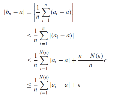
  To continue, we use a simple analysis result (Cesaro mean): if $a_n→a$ and $b_n = \frac{1}{n} \sum_i^n a_i$, then $b_n →a$. This is a simple epsilon proof

  • proof

    

  Now, from the chain rule, we know that

  

  let LHS be $b_n$. We know that $a_i → H’$, so by the Cesaro mean theorem, we have

  

  as desired.

Markov Chains

In the AEP section, we talked about IID variables, which is a good start, but we seldom deal with IID characters in real life. Here, we move to another level of complexity, where we have random variables that satisfy the Markov property.

The best way of thinking of a Markov Chain is as as journey of samples, in accordance to the Markov probabilities. You record this sample down as the stochastic process. You look at general behavior: what do a distribution of such samples look like? At the end of the day, it’s just a joint distribution with special properties.

PGM view

Markov chains are just PGMs such that every pair in the PGM has only one active path.

The key idea

If you took a random slice of a markov chain, you get some random variable $X$. This $X$ can be distributed like anything. If it’s in the stationary distribution, then any $X$ slice shares the same distribution statistics. Now, even though every slice shares the same statistics doesn’t mean that it’s IID! There is a dependence, which is captured by the $p(x’ | x)$.

Therefore, you might have two $X_1, X_n$ that are all identically distributed, but they have a dependence.

Markov Properties 🐧

Remember that the markov property means that you can factor the joint distribution as so:

which means that you can express the following relationships between samples:

Intuitively, we’re just making a joint distribution and marginalizing. This is also equivalent to $Pu$, where $u$ is a vector of probabilities that represents $p(x_n)$.

Markov chains are time invariant if $p(x_{n+1} | x_n)$ is agnostic to $n$. This is different from being stationary (more on this in a second). We can express the a time invariant Markov chain through a matrix where $P_{ij} = P(X = i | X = j)$. All columns of the matrix sum to 1. Matrix multiplication $Pu$ is just a weighted sums of the columns, which is guarenteed to be a distribution.

The Matrix

The matrix $P$ is quite special.

• If the markov chain has a stationary distribution, then it has an eigenvector with value $\lambda = 1$.

• Repeated powers of $P$ converge to the stationary distribution, where every column represents the stationary distribution. Why? Remember that matrix multiplication is also seen as taking the weighted combination of columns. This means that $P^\infty u = S$ for any $u$, where $S$ is the stationary distribution

• You can easily calculate $p(X_n = a | X_1 = b) = (P^{n-1})_{ba}$. This can be proven by doing the standard marginalization. The marginalization is exactly the same as matrix multiplication in this case.

Special Properties 🐧

• If we can get to any arbitrary state from any arbitrary state (i.e. there’s no “death” state in between), the Markov Chain is irreducible.

• If you can group the states non-trivially such that all transitions flow from one group to another, then the Markov Chain is periodic. As a concrete example, If you had $A → B$ and then $B→A$, then it is periodic with $d = 2$. In contrast, if you had $A→ B$, $A→C$, and $B$ had no connection back to $A$, it is aperiodic. More formally, if the largest common factor of the lengths of paths from states to themselves is $1$, then it is aperiodic.

• If $p(x_{n+1}) = p(x_n)$ (note their relationship from previous section), then the distribution at time $n$ is stationary (drawn directly from the definition of a stationary distribution)

If Markov chain is irreducible and aperiodic, then the stationary distribution is unique and a convergence point.

You can solve for convergence points by using the vector definition: $u = Pu$. Usually, this gets you an equation that can’t be solved directly (it’s underdetermined) but you can use the final constraint that $\sum u = 1$. When you solved for all $u$, you have a stationary distribution!

Entropy of Markov Chain

In general, you can find the conditional entropy by using the vector definition.

and this is taken directly from the definition of conditional entropy and the meaning of $P$ and $u$.

Entropy Rates

As long as the distribution is stationary, then

So the limit is just $H(X’|X)$, where we draw from the stationary distribution. We can calculate this value by using the stationary distribution and then the $p(x | x)$ of the Markov matrix.

• Alternative derivation