Convergence of Random Variables

What is a sequence of random variables? Well, maybe think about dice that come out from a dice factory. Each dice is an RV, and there may be a pattern in how the dice behave.

There are different notions of convergence.

1. in distribution means that we converge to the same sufficient statistics

2. in probability means that for every $\epsilon > 0$, we have $p(|X_n - X| > \epsilon) → 0$. Intuitively, the probability of an “unusual” outcome becomes more rare as sequence progresses. Close to the idea of a hoeffding’s inequality, useful for the law of large numbers, etc.
   1. with this inequaltiy, you can say that we asymptotically bound this property within an epsilon ball
   2. Formally: for every $\delta$, there exists some $N(\delta,\epsilon)$ such that for all $n > N(\delta,\epsilon)$, we have $p(|X_n - X| > \epsilon) < \delta$. Note how this $N$ depends on both the delta and the epsilon.

3. in mean square if $E[X_n - X]^2 → 0$ as $n → \infty$.

4. with probability 1 (almost surely) if $P(\lim X_n = X) = 1$.
   1. this is different from 2) because we take the limit inside the probability.

Notation-wise, we use $X_n \overset d\rightarrow X$ for distribution, $X_n \overset p \rightarrow X$ for probability, etc.

Understanding what convergence means

Distributional convergence makes sense. But how can the other types of convergence happen if these are random variables? Well, there are two common cases:

1. The $X_n = f(X)$ DIRECTLY, and $f_n → 1$ as $n→\infty$. In other words, there’s some sort of coupling between the RV’s.

2. The $X$ is a constant. Here, we get some standard things like the central limit theorem, where $X = E[X]$ (overload of notation), and $X_n$ is the mean of the current samples.

Markov’s Inequality

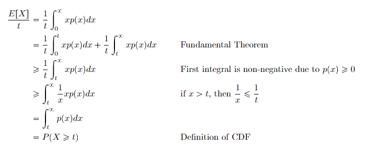
We can show that for any non-negative random variable $X$ and $t > 0$, we have

Intuitively, as we get further away from the expected value, the likelihood decreases. This is mathematically super helpful as it relates probabilities to expectations, and we will use it to build up law of large numbers.

• Proof (integral definition of probability and expectation)

  

Chebyshev’s inequality

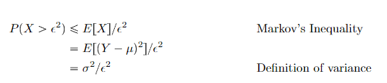
We can show very easily that

where $\sigma^2, \mu$ is the variance and mean of $Y$, respectively. This brings us closer to the idea of hoeffding’s inequaltiy and the law of large numbers.

• Proof (Markov’s inequality)

  Let $X = (Y - \mu)^2$

  

Upshot: to show the law of large numbers for any stochastic process, it is sufficient to show that the variance of the sample goes to zero.

Law of Large Numbers

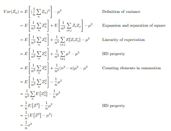
Lemma: Sample variances

The variance of $\frac{1}{n}\sum Z_i$ is $\sigma^2 / n$

• Proof (from definitions)

  

The actual Law ⭐

Both the weak and strong forms of the law of large numbers state that the average of samples (denoted by $X_n$) converges to $E[X]$.

The weak form states that the convergence happens in probability. Formally, this means that

• Proof (Markov’s inequality and sample variances)

  Let $X = (\frac{1}{n}\sum X_n - E[X])^2$

  

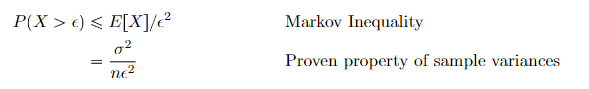
  which gets us

  $$P(\left|\frac{1}{n}\sum_nX_n - E[X]\right| > \epsilon) \leq \frac{\sigma^2}{n\epsilon^2}$$

  and as we can see, the limit of the RHS pinches to 0, and that is what we wanted to show.

The strong form states that it happens almost surely. Proof is omitted for now.