Proof tips

• Expand $I(X;Y) = H(Y) - H(Y | X)$ as we know $p(y|x)$.

• If confused, try adding a weird state directly into the entropy and removing it through chain rule.

• $H(Y)$ is a convex function of $p(x)$ for any given $p(y | x)$. Convexity in this case means treating the distribution like vectors.

• If it doesn’t work on first expansion, try a different expansion

• for matrices, make sure to watch out: if the rows sum to 1, you can’t do matrix-vector multiplication

Moving to Noisy Channels

Now, we are graduating onto channels that have noise, i.e. you send in some $x$ and you get $p(y | x)$. What does that look like? Well, previously we had info → encoder → decoder → info. Now, we need info → encoder → channel encoder → NOISE → channel decoder → decoder → approximate info

The Assumptions

Our job is to make this meaningful channel encoder and decoder.

IID Uniform inputs: Fortunately, we can actually make a key assumption about the data going into this set of encoders. Because we assume that we have a good data encoder algorithm, we can assume that the input is binary RV’s that are IID. Why IID? Well, if the variable had any sort of correlation, we can further compress until they are maximally orthogonal, in terms of probability.

By assuming that the input and output are just binary streams, we can actually start thinking about them as numbers that these binary things represent. Our goal is to send one number and reconstruct it as accurate as possible.

Discrete and Memoryless Channel (DMC): we can assume that the noise is memoryless, i.e. $p(y_1, .., y_m | x_1, …, x_m) = p(y_1|x_1)…p(y_m|x_m)$. This is very similar to an IID assumption.

The channel goes $W → X → Y → \hat{W}$. We can’t assume any IID of the X or Y.

Nomenclature

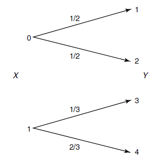
We use an arrow diagram to denote the distributions over outcomes, which can be helpful to visualize thing

Performance Metrics

There are two things we care about

1. Reliability: Can we have $P(W \neq \hat{W}) = p_\epsilon << 1$? (where $W$ is the whole message)

2. Rate. Can we maximize the number of information bits per channel symbol?

Intuitively, these two metrics are battling. You can easily get a very reliable code if you have a really redundant signal, but this tanks your rate. Vice versa. In a later section, we will look at how these things aren’t necessarily competing if we do things correctly.

Channel Capacity

Why we can’t just take the percentage of mistakes

So the big question is: how do we quantify how good a signal is? We can’t just subtract the average number of mistakes, because you can have a channel that is maximally uncorrelated with the input, and still not make a mistake 50% of the time (just by pure chance, if you guess a binary digit, it matches the source 50% of the time). Furthermore, sometimes you lose more than the average number of mistakes, as you don’t know where the mistakes are.

Moving to capacity

Instead, it helps to think about the correlation, or mutual information between the source and the output.

There’s something interesting about this setup. Mutual information depends on $p(x, y)$, which is factored into $p(y | x)p(x)$. Now, $p(y|x)$ is a property of the transmission system. It’s $p(x)$ that you can modify.

Therefore, we define capacity as

As we will see, there’s a strategy in how we design $p(x)$. We want to have each $x\sim p(x)$ to map to as far separated $y$ as possible, such that the inverted $p(x | y)$ is as noiseless as possible. This is actually a concave function because $I$ Is concave in $p(x)$.

Meaning of capacity

Interestingly, this $C$ has a key meaning: below the rate of $C$, you can send information with as high of a precision as possible!

We will prove this fact in the next page of notes.

Properties 🚀

• non-negative (due to mutual information)

• $C \leq \log |X|, \leq \log |Y|$ because $\max I(X;Y) \leq \max H(X) = \log |X|$ and vice versa

• continuous

• concave (but no closed form solution, typically. We use other strategies to get it solved)

How to optimize 🔨

So this objective is not very easy to optimize directly. You can use a few tricks

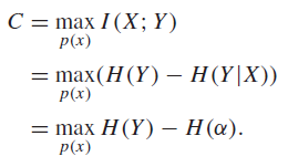
1. $I(X;Y) = H(Y) - H(Y | X)$. This is helpful because $Y$ is maximized through a uniform distribution, and $H(Y | X)$ is often easy to derive.

2. Now, the tricky part is to figure out (often) how to create a maximum entropy $Y$ using $X$. You might benefit from $I(X;Y) = H(X) - H(X | Y)$, which gives you a more direct formulation. The only problem is that the $H(X | Y)$ is now convoluted.

3. You can also brute-force. Start with a representation of $p(x) = [p_1, p_2, …, p_n]$. If you have a conditional probability matrix, $P$, then $p(y) = P[p_1,p_2, …p_n]$. Using $P$, you wil also be able to derive $H(Y | X)$. Usually, this sort of brute-force optimization is messy and requires some sort of crucial insight. But it can be helpful to set it up this way.

What is rate? Capacity?

Rate is the number of message bits per channel bit. Capacity is also measured in the same units, and can never exceed $1$ for binary channels. This is mathematically true because the Bernoulli RV $H(X) \leq 1$.

Rate is determined in the encoder, i.e. the transfer from $W → X^n$. The capacity is determined by the $X → Y$ channel. The theory we develop will relate the rate to the capacity.

Example of Noisy Channels

Noiseless binary

Here, we consider a degenerate case where we have no noise at all. In this case, $\max I(X ; Y) = \max H(X) - H(X | Y) = \max H(X)$, which is maximized with a uniform $p(x)$.

Non-overlapping outputs

Consider the following distribution (repeated from nomenclature diagram):

This looks noisy, but actually, $p(x | y)$ is noiseless. So the channel is also maximized with a uniform $p(x)$. This is a good example of how the $H(X) - H(X | Y)$ expansion is critical.

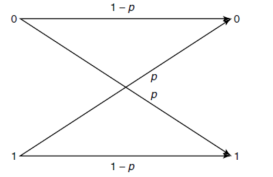
Binary Symmetric ⭐

Here, the inputs are complemented with probability $p$. So everything that we receive is unreliable, but that doesn’t mean that we can’t send anything. We’ll see an algorithm later.

We can show that binary symmetric mutual information is bounded by $p$: $I(X;Y) \leq 1 - H(p)$. If $p = 0.5$, it is impossible to carry any information.

• Proof

  

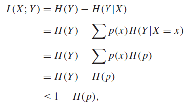
  Two tricks: 1) we discovered that the second term doesn’t depend on $p(x)$, so we are off the hook. 2) we assert that it is possible to achieve $H(Y) = 1$ by feeding in a uniform input, by symmetry. These are two tricks that are specific to this problem.

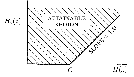
Now, this has some interesting implications. At any given $p$, there are $1-p$ bits of information left uncorrupted. However, if you plot the line $1-p$ vs $1 - H(p)$, you will find that the curve of $C$ goes below the $1-p$. This is intuitive; it means that by randomly flipping some bits, you lose more than just the proportion of bits you flipped, because you don’t know where they got flipped.

• Properties of $X, Y$ (can be important)

  The input is Bernoulli, the bit-flip is Bernoulli, so the output is also Bernoulli. If input is $Ber(p)$ and flip is $Ber(q)$, then the distribution is $[pq + (1-p)(1-q), p(1-q) + q(1-p)]$, or $Ber(pq + (1-p)(1-q))$.

  The conditional entropy $H(Y | X)$ is the same as $H(q)$, because the entropy of $Y$ does not depend on $X$ (hence the symmetry). Therefore, $H(X, Y) = H(p) + H(q)$. Nice! This makes a lot of sense.

Binary Erasure ⭐

Here, instead of corrupting bits, we just lose some bits with probability $\alpha$

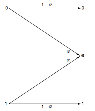
We can actually derive exactly what $C$ is: $C = 1 - \alpha$. This is intuitive, because if we lose $\alpha$ proportion of bits, we can only recover $1-\alpha$ bits.

• Derivation

  So this structure yields something hairy, because there’s this death state, essentially. We can start with this original expansion

  

  But how does $H(Y)$ depend on $X$? And is the maximum $\log 3$? So actually, we can never get to $\log 3$, out of a simple principle: you can’t gain entropy by passing through a varible. The source variable $x$ has maximum entropy of $1$.

  So in this case, we actually benefit from the opposite expansion. We know that $H(X | Y) = \alpha$, and it is agnostic to $p(x)$. Therefore, we can maximize entropy with a uniform on $X$

  $$I(X;Y) = H(X) - H(X | Y) = 1 - \alpha$$

Interestingly, this channel is able to preserve in communication the average number of bits kept untouched, unlike what we saw in the binary symmetric channel.

Symmetric Channels (extra)

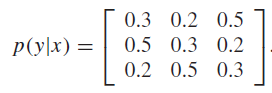
Consider a more general form, where we have $p(y|x)$ as a matrix

What can we say about the channel limits now?

Symmetric definition 🐧

Now, in the example above, we notice how the rows are permutations of each other, and so are the columns. We call this a symmetric channel. Intuitively, it means that the entropy of the output doesn’t depend on the input, but the distribution does.

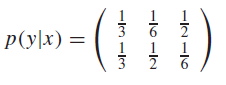
If the rows are permutation and the column sums are equal, then it is weakly symmetric

• Example of weakly symmetric D

  

Channel Capacity

We can find the channel capacity by performing the following standard derivation

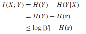
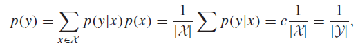
And we can maximize $H(Y)$ by feeding in a uniformly distributed input

• Proof (factor)

  

And this is true for weakly symmetric inputs as well