Noise Free Coding Algorithms
| Tags | EE 276Noise |
|---|
Moving from Theory
So in the original formulation, we showed that any random code can yield an error that goes to 0, as long as the rate is smaller than the capacity. But a random code is very bad! It is exponential in encoding and decoding (especially in decoding). Can we do better?
Linear Codes
Let’s go back to a string of bits. We represent and . What if we have some matrix in a finite-field of size 2 (i.e. it’s a bunch of 1’s and 0’s, and when you do matrix multiplication, you do mod 2), such that ?
The encoding process you can imagine as creating a system of equations and sending a linear combination of inputs. The decoding process you can imagine as solving this system. If you create enough overdetermination, you will be able to solve the problem even if the signal becomes corrupt.
Linear Codes on Binary Erasure
The Binary Erasure Channel is the easiest example for how Linear codes work. If we have and the channel erases some of the we are just left with a lower number of linear equations. As long as these equations are enough for one unique solution, we can still decode the original message.
How do you choose G? Well, you can just choose it randomly, and it’s possible to show that this is optimal with high probability.
Efficiency
The encoding is very simple: it’s just the complexity of matrix multiplication. Decoding is slightly more tricky: it requires an inversion of a matrix.
Intuition for why rate matters: linear codes
this is an additional section but it can be helpful to get us to understand why we care about rate . We know that there are bits in the message and bits in the code. In our case, . Let’s assume a random code where every is mapped randomly. And let’s assume that the channel itself is noiseless.
- The chance of individual error is becuase there are this many codes.
- There are words. So the union bound states that . This is the average error probability per bit. If , we see how will push this error probability to 0. Why? Intuitively, there’s more space than there are words, so we can find ways of separating
- If there are words (), we run into interesting land. Using complements, we can calculate that the probability of no error is , which limits to . This means that there will always be some probability of error, which makes sense. There is no gap that is growing larger.
Proof of functionality
The tl;dr is that any matrix multiplication of G is just a summation of IID vectors, which is IID. Then you can plug this argument into the random code argument. The slight caveat is that the case is not uniformly distributed. This is only one point, so it is fine.
Polar Codes: The Theory
The big idea
For simplicity, let’s say we have IID Ber(0.5), which is our message. We pass it into a coding scheme , yielding , and then into the channel to yield . Under the current system, the ’s get encoded in to and then get sent through one type of channel. Therefore, the noise is “distributed” across the .
In polar codes, we want to shift the noise such that it is asymmetrical. We have some bits of with very low noise (i.e. very easy to figure out after transmission) and other bits that essentially only act as checksums. (this is why the code is called polar: because things get pushed to opposites).
The Assumptions
- Standard pipeline
- The coding matrix is full rank (no loss of information)
- is IID uniform, and any linear transformation of is still uniform (because is invertible)
The Encoder G
Let’s start with the simplest case where there are only two bits. We do this because we want to show a fundamental property that allows us to construct arbitrary sizes.
Because we assume that is full rank, there is really only one option (and its symmetric option):
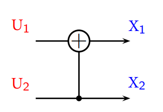
And because we are dealing with finite field of size 2, we can actually represent this as the following diagram:
In fact, all can be represented as a collection of these XOR gates (just think about it for a second). The capacity of the channel with is , where is the capacity of .
Building up the Polarizer: the Chain Rule
Now, the capacity is , and every bit contributes to the capacity. Can we somehow polarize this, such that one bit has more capacity than the other?
Well, note that
This creates two separate channels!
The first channel
The first channel looks like this:
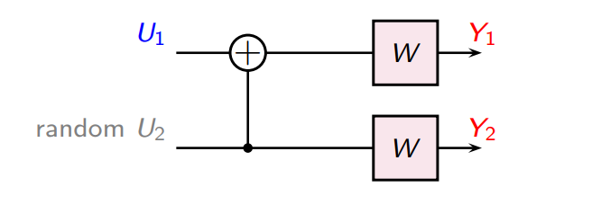
We are trying to infer from . In this channel, is just noise.
The second channel
The second channel is a bit more tricky, because we don’t know what the conditional MI means. However, from the chain rule, we get
And we know that the U’s are independent, so . So, our second channel looks like this:
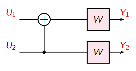
Now, this is just a repetition code! We are trying to infer from .
Here, we note that this might seem weird that the channel feeds back to predict . In reality, we don’t care bout the , but we do care about the .
Intuition about the two channels
The first channel is between and . Intuitively, you make a prediction on , and then you graduate onto the second channel, which is between and . This means that you’ve gone ahead and observed and let it be part of your decoding input.
The idea of these two channels is that we build up the next channel using the we’ve already used.
More generally, it’s possible to show that
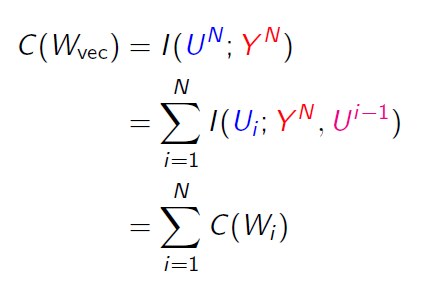
which shows the recurrent relationship.
As an alternative intuition, you see how the less noisy channel relies on the more noisy channel almost as a checksum. Polarization is just the assignment of certain channels as checksums of the other channels.
Polarization Theory
It is possible to show that
Or in other words, we will reach maximum polarization, at which point the proportion of non-zero capacities will be equal to the capacity.
Martingale
So the idea is that with larger enough chunks, you will get a lot of high capacity channels and a lot of low capacity channels, and very little in-between. The proof is more complicated and requires martingale, but you can imagine this as a random walk. On each step, you either take a step right or left. If you are bounded on either side by a wall, most of the random walks will end up stuck along that wall.
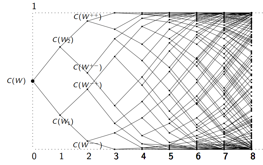
The Polarizer on BEC: Case study
We can show polarization really easily on a binary erasure channel. Let’s say the erasure probability is .
- the first channel requires both to decode because of that XOR. So, if either one is flipped, we essentially erase everything. So, this new channel is also BEC with erasure probability
- The second channel is a repetition code, so it requires both erasures to render the information irrecoverable. So, the new channel is also BEC with erasure probability .
For a binary erasure channel, . You can easily tell that the first channel has capacity , which is smaller than unless the (trivial cases). And , so , and therefore the second channel has higher capacity than .
We can continue to extend this result recursively. You can imagine the general rule
- Enrich channel: take the old parameter and create new
- Deplete channel: take the old parameter and create new .
Polar Codes: The Implementation
General polarization
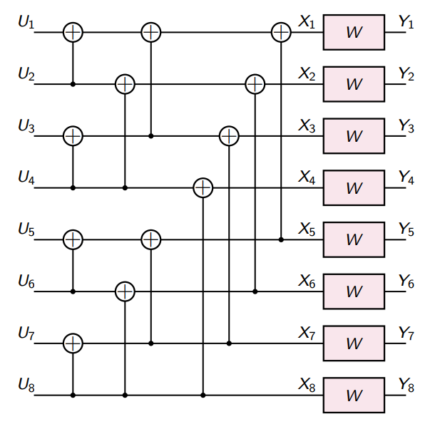
We just apply the Polarization algorithm to the positive and the negative channels after initial polarization. This yields . Keep doing this until there are channels.
Example on 4
First, create two pairs of channels
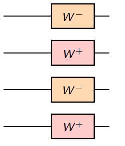
Then, treating the matching pairs as identical, apply the basic transform
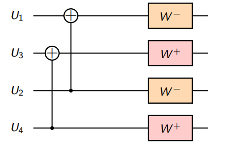
We get the new channels
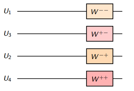
And so this looks like
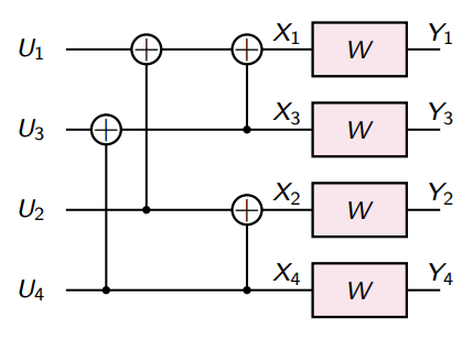
The construction continues recursively. The final result is that you get a bunch of XOR operations that you can turn into a matrix.
Encoder
We’ve already gotten a hint on how to use the polarizer. We can continue to run the polarizer on its outputs. This creates a tree of channels with different properties. But this is all in theory. How exactly is this done?
Well, to strip it all down, it’s actually just , where has a special structure.

You can construct things recursively and do matrix multiplication, but this is . Can we do better?
Yes! We can compute the matrix multiplication using recursive computation through block matrices. Consider this:
So this becomes a previous recursive case and vector addition. The vector addition is , so the total complexity is . But in general, encoding is matrix multiplication.
When you decide to fix some subset of as 0, it’s equivalent to removing those columns of . So the final encoding is just a missing the columns that you chose to remove.
Decoder
Ultimately, you want to compute The base cases: , and . If you look at the way that the G is constructed, you can always find the outermost modified W’s that form a single one-step polarized channel. You only need to unpeel a certain subset of these connections and it reduces down to a self-similar problem. The exactly mechanisms is pretty hairy, but know that it is recursive and runs in O(n^2) time.
Visually, it’s a forward backward process.
