Proof tips

• usually you can expand things twice, which gives you an automatic relationship (true for anything with the chain rule)

• use indicator variables as bernoulli RV’s

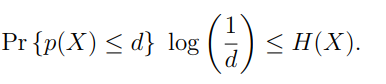
• upper bound probability of event $X$. If you think of $X$, does it entail event $Y$? And does this event $Y$ have an easily expressible form? If $X$ implies $Y$, then $p(X) \leq p(Y)$.

• always start from basic definitions; it helps a ton

The Basics

Notation

Sometime we use the $Pr\{\}$ notation if using another $P$ is confusing. This is common for CDF, or if the likelihood is a random varaible

• we use CAPITAL to represent the random variable itself. So $p(X)$ means a random variable $X$ such that we run it through the probability function $p$ after sampling
  • general rule of thumb: if it’s outside of a summation, and you just want to refer to “something”, capital is the way to go.

• we use lowercase to represent a sample or an instance. So $p(x)$ is a number (shows up in summations, etc).

Proof techniques

• To show that $f(x) > g(x)$, you can show a few things. You can show that their differnce is positive / negative
  • for differences: compute the first derivative to find the maximum difference or minimum difference. compute the second derivative to see how many extrema you need to test for
  • the concavity argument: if $f(x) = g(x)$ at one point and $f’(x) \geq g’(x)$ at this point and $f’’(x) \geq g’’(x)$ for all $x$, then you can say that $f(x) \geq g(x)$ for all $x$ after that one point of equality.

• dead end? Try something new!

• Always feel like you can justify from first principles.

• sometimes you need to go both ways: there are some facts you know directly from some inequality, and then you move your way backwards to get your final product. For example: you know that $x > y$, and then you know that $z > x$, so you can conclude that $z > y$.

• Simple tricks work best for minimally constrained problems

• add and marginalize is a really big one too

• To show something about $Pr(x \in X)$, you can use this: $\sum_{x \in Y} p(x)$. Simple trick but the latter gets you to something that you might be able to calculate

Limit behavior

• $\lim_{x→0}x \log 1/x = 0$. Intuitively, this is true because one pinches linearly and the other explodes logarithmically

• If you want to know what happens to $f(x, y)$ as $x, y \rightarrow \infty$, you need to replace it with one variable (i.e. you need to find a relationship between $x, y$. Two-variable limits are not totally well-defined unless this replacement is done.

• $\lim_{x →\infty} (1 + 1/x)^x = e$, and by symmetry we have $\lim_{x →\infty} (1 - 1/x)^x = 1/e$

Summations

Raising a summation to an exponent is the same as nesting exponents. This goes to a deeper truth that

which is intuitively true because multiplication does pairwise, and nested sum also does pairwise.

Fractions

• The $a / (1-a) = c$ trick always yields $a = \frac{c}{c + 1}$, although that sometimes isn’t the best form. Always look for ways of simplifying that remove the extra 1.

CDF

If you have something like $p(x > k)$, this is an integral over the PDF. If you’re dealing with discrete things, just take the summation (discrete there’s no notion of PDF).

Expectations

• remember that expectation is an integral. You can’t switch any non-linear function with an expectation (although Jensen’s can give you an inequality)

• If $X, Y$ are independent, then $E[XY] = E[X]E[Y]$.

Marginalization

You can marginalize distributions, but you CAN’T marginalize something like $H(X, Y)$. This is because we already take the joint expectation and the entropy operator is not linear.

• Instead of marginalizing, consider chain rule

But…marginalization is your most common tool. If you want to calculate some $p(x, y)$ but it’s easier for you to calculate $p(x, y | z)$, then do $\sum_z p(x, y | z)p(z)$.

Chain rule

It can be easy to forget the actual chain rule. Remember: $p(x, y) = p(x | y) p(y)$. The variable only appears on the non-conditional ONCE. It does not appear again, or else we run into problems.

“p”

Here’s also a point of confusion that sounds stupid but it happens all the time. The $p$ is not a specific function. So $p(x | y)$ isn’t the same as $p(a | b)$, etc. This is true even when the $p$ is specialized for some application. Probability is not a function.

Hard constraint inequality

If I have $X + Y = C$ and I know that $Y < B$, what can I say about $X$? Well, I know that $X = C - Y$, and this is the tricky part: we know that $-Y > -B$, so $C + (-Y) > C + (-B)$. So, $X > C - B$. The inquality is flipped. This is also true by vibes. A common mistake is the switch the location of the $Y$ without flipping the sign of the inequality.

Advanced properties of RV’s

The formal definition of density

So for continuous RV’s , we have the notion of density $f(x)$. When defining the density, we always do it in terms of the CDF $F$.

so this is a great first step when you’re dealing with proofs with density. And of course, remember that

and you can apply functions inside the $p$, like $p(\phi(k) < x) → p(k < \phi^{-1}(x))$.

Information lines vs dependency lines

In things like Markov chains, we draw things like $X → Y$. In communication, we might draw something like $X -[P]- Y$. What is the difference? Is there a difference?

• The $-[P]-$ indicates that there is something that messes the signal up between $X$ and $Y$. Depending on how bad it is, $I(X ; Y)$ could range from 0 to some positive number.

• The $→$ is a more vague version of this $-[P]-$ notation. We just know that there is a dependency, a distribution $p(y|x)$. This could be the same as $p(y)$, although it is generally good practice to remove the arrow if that’s the case. So there’s a subtle difference. If $X →Y$, then we know that $I(X ; Y) > 0$.

Densities

The density $p(s)$ means the likelihood of $s$, which ALSO means that if you were to select $s$ at random, the likelihood of $s$ being this current $s$ has likelihood $p(s)$.

Remember that $p(s)$ is a value, as $s$ is scalar. Therefore, $p(s | v)$ is well-defined, but NOT $p(s | V)$. The conditioning must always be deterministic. On the other hand, $p(S | v)$ is totally fine; it’s just another random variable.

What is a random variable??

A random variable $X$ is nothing more than a tuple containing $p(x)$ distribution, and a range $\chi$. This $x$ in $p(x)$ indexes into $\chi$, but that’s only an indexing property. So…as long as you have some set $\chi$ and a valid probability distribution with the same cardinality, you’ve got yourself a random variable.

• Example

  As an example, we can have $q_i$ be the $\chi$ and $b_i/\sum b_j$ as the $p(x)$. Note how $b$ and $q$ can have no relation. As long as they have the same cardinality, it is possible to make an RV out of them.

Convexity in a distribution

This is definition a mind trip, but certain things can have convexity or concavity WRT distributions. Don’t get too confused. A distribution is just a vector with L1 length 1. You can interpolate between two vectors, whose intermediate vectors are still L1 length 1. This interpolation is the secant line drawn between two distributions.

Linear function of a distribution

When we have something like $\sum_x p(x) g_x$, we say that this is a linear function of $p(x)$. Again, back to our view that a distribution is a vector. This is the same as doing a Hadamard product on the vector, which is linear.

Same RV, same parameters

Here’s a critical distinction. When we talk about some RV $X$, it has an identity as well as parameters. If we set $Y = X$, this means that every sample of $Y$ is the same as $X$.

However, there’s also the notion of sufficient statistics. If we have $p(Y = y) = P(X = y)$, then we have the same distribution, but the identity of $X, Y$ are not the same. As a consequence, if you draw a sample from X, it may not be the same as the sample from Y.

Distributions over likelihoods

So $X$ is a random variable, and $p(X)$ is also a random variable. This is because $p$ is just a function that takes in something and outputs a number between 0 and 1. Therefore, $p(X)$ is feeding the sample back into its own likelihood fuction. This is perfectly valid, and in fact, this is exactly what entropy does! $E[\log 1/p(X)]$.

Union and intersection bounds

This is basic stuff but it can be very useful

• “at least one”: use a union, which is upper bounded by the summation of probabilities and lower-bounded by the single largest probability

• “all of them”: use an intersection, which is upper-bounded by the smallest probability. For the lower bound is a bit tricky. $P(A \cap B) = P(A) + P(B) - P(A\cup B)$. If $P(A) + P(B) < 1$, then we can make them maximally separate. If $P(A) + P(B) > 1$, then there must be some intersection. So $P(A \cap B) \geq P(A) + P(B) - \min(1, P(A) + P(B))$

Remember that “not one” is equivalent to “all of them” (the laws of set negation).

Transforms of random

This is kinda tricky. If we have an invertible matrix $G$ and a uniform random vector $u$, then $Gu$ is uniformly random. Why?

Well, if $u$ is uniform, think about the VECTOR not the scalars. This $G$ will map $u$ to $v$ in a one-to-one manner. So, the G is just reshuffling the random.

There are also special properties when we are in $F_2$. Namely, adding random uniform vectors make more random uniform vectors because addition is equivalent to bit flipping. This is not true for real-valued vectors. Adding uniform RV’s is equivalent to a random walk, and there are some deeper theories about this.

• and as such, if you have any random uniform matrix $G$ and multiply it by some $u^k$, then every output will be random, as every output is a different sum of random uniform columns.

Splitting and moving in entropy, MI, etc

• to split before conditional, consider using any chain rule

• to split after conditional, consider using mutual information, which breaks $I(X;Y) = H(X) - H(X | Y)$, which gives you essentially the “chain rule” but on the other side of the conditional

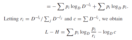
Making distributions from nothing at all

When you’re faced with something that feels very close to a distribution, feel free to multiply by the sum and divide by the sum. Division by the sum makes the thing into a distribution

• Example

  

Some tips for spotting wannabe distributions

1. summations with indices (just divide by the summation to get a distribution). Often, you can make the summation into an expectation of something WRT a distribution .

2. things with logs and inequalities (because with a distribution, you can use Jensen’s inequality)

Why do this? Well, things like Jensen’s inequalty and expectations don’t work without a distribution, so it’s beneficial to make one.

Writing distributions as charts

• joint distribution: whole thing sums to 1

• Conditional distribution: column or row sums to 1

• computing conditional from joint: normalize across a column or row

It’s tricky keeping track of what is what sometimes! Good labeling is always key.

Martingale

A martingale is a stochastic process where the expected next state is the same as the previous state. Or, in mathematical terms

A good example of a Martingale is a random walk. This is a bit beyond our paygrade, but Martingales have certain interesting properties that we can use to our advantage.

Change of variables

Suppose that you have $y = q(x)$ where $q$ is invertible and differentiable. You eventually want to integrate along $x$, but perhaps the formula is simple in $y$ space. So you start in $y$ space. For the sake of this problem I’ll just be doing a simple integral.

Oh, but this is weird. How do we integrate over $q(x)$? Well, we know that $dy = q’(x)dx$, so this just becomes

which hopefully is reminiscent of u-substitution. And then you just integrate over $x$.

General strategy when dealing with change of variables: know how these are related on the non-derivative but also through the derivative $dx, dy$ so that you can connect them.

Finding f

In the derivation above, we just assume that $f$ existed naturally. Now, typically for distributions, you have some $p(x)$, some transform $y = \phi(x)$, and you might want to find the quanity $h(y)$, which is easier to do in y-space first, but that you require you to find some $g(x)$ equivalent of density in Y-space. Now this is actually not trivial. You start from first principles:

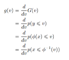
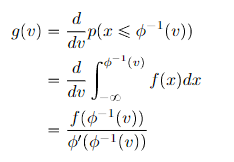
Note how you divide by this derivative term. This is a result of the density definition.