Gaussian Channels

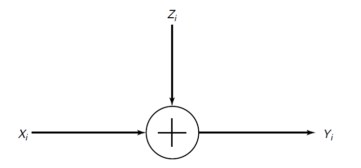
The gaussian channel is just a continuous RV with an added noise vector

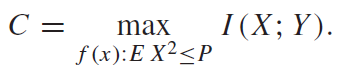
Of course, if $X$ weren’t constrained, the capacity is arbitrarily large because you can essentially make $X$ as large as possible to drown the noise out. So, we are interested in situations where the $X$ has a certain limit:

where $P$ is the power limit.

The channel

We make a power-constrained channel as follows

And we can use the chain rule of MI and the knowledge that $Y = X + Z$ to yield the following derivation

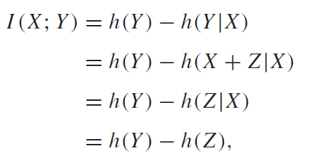
We know the closed form expression for $h(z)$.

Now, we continue by realizing that $Y = X + Z$. We know that $E[Y^2] = E[X^2] + E[Z^2] = P + \sigma^2$ because they are independent and $E[X], E[Z] = 0$. Now, this is actually really nice. We know that a gaussian maximizes this second moment, so $h(y) \leq \frac{1}{2}\log (2\pi e(p + \sigma^2))$. But is this gaussian achievable?

As it turns out, yes! The sum of two independent gaussians is gaussian, so we can just use the maximizing distribution for $E[X^2] \leq P$, which is the gaussian with variance $P$. If we add this to $Z$, we get the maximizing distribution for $Y$. In this case, we have

And this is the capacity of a gaussian channel! We call the $p / \sigma^2$ the signal to noise ratio, and we see how the capacity depends on it.

Quantized Gaussian

You might let $X$ be a binary signal. This gets you a quantized channel with the $Y$ being a bimodal gaussian. This reduces the capacity (still by symmetry, the $X$ should be uniform).

You might further choose to quanitize the output $Y$. At this point, you have created a BSC with crossover probability $p$, which is a function of the power limit and the noise of $z$. You calculate this by taking the CDF.