Proof tips

• chain rule! Always helpful
  • for MI, it is helpful because you can express things two ways
  • for MI, it is also helpful because it will allow you to introduce another variable

Big chart of conditions, functions, etc

Entropy

Definition 🐧

Mathematically, it’s defined as

We denote $H_b(X)$ as the entropy WRT base $b$, although by the change in base formula it’s just shifted by some constant. Entropy is measured in bits, if you use base 2 (which is the most common)

The logarithm function is actually not completely necessary; it just gives a nice mathematical property and also relevant to communication

The key intuition

You can understand entropy as the average information gained after seeing a sample from a RV. “information” is basically the “surprise” you get from seeing the sample. Another way of understanding entropy is uncertainty

• If the RV is deterministic, then you gain no information from a sample, so entropy is zero

• If the RV has a very clear mode, then the entropy is low, because most of the time you get the mode and you get little information. When you don’t get the mode, the information is larger, but it’s also rare that you land outside the mode

• If the RV is uniform, you get the most information from a sample (previously, it could have been anything with equal probability!) ‘

You can also understand H(X) as the average bits needed to represent X.

Key properties 🚀

• Entropy is non-negative. Proof: probability is always ≤ 1, so negative log is positive

• Entropy is label invariant. In other words, it doesn’t matter what values the RV takes on; as long as the probability distribution stays the same, the entropy doesn’t change. Or, in mathematical terms, if you have an injective function $f(x)$, then $H(f(X)) = H(X)$
  • Corollary: Entropy is highly symmetric. The symmetry comes from this invariance
  • General statement: $H(f(X)) \leq H(X)$ for any function (suppose you map non-injectively)

• Entropy is bounded by the number of elements: $H(X) \leq \log |X|$
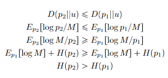
  • Same thing: Entropy is always maximized at the uniform distribution.
  • Proof (non-negativity of conditional entropy)

    The idea is to take the KL divergence between $p$ and the uniform $u = 1 / |X|$.

    

    And we know that this is ≥ 0, so we have $H(X) \leq \log |X|$, as desired.

  • Stronger claim: the closer we get to uniform, the larger entropy gets (monotonic)
  • Proof (KL)

    

• Entropy is concave in p
  • Proof (convexity of KL)

    Use the same trick as above. If you write out $D(p || u)$ and massage it, you get

    

    and we know that KL is convex, so the negative is concave. The log is a constant and doesn’t matter.

From first principles

There is a common question of why entropy is actually written in this form. It turns out that it was defined under 3 constraints.

1. If we have a uniform distribution, H is monotonic in n, the number of categories

2. If we split the distribution, the entropies should be the weighted sum

3. H should be continuous in $p$

There are other functions that work, but the log is the cleanest.

Aside: Cross Entropy

Cross entropy is the same as entropy, except that we take the expectation under a different distribution

Intuitively, if we are going back to our bits example, the cross entropy is the number of bits you would use to represent distribution $Q$ if we used the optimal encoding scheme from $P$.

Joint Entropy

The definition 🐧

We define the joint entropy as just the entropy of multiple variables

This is nothing special, as you can treat $X, Y$ as one random variable. And indeed, you can see very easily that if $X, Y$ are independent, then $H(X, Y) = H(X) + H(Y)$.

Independence bound on Entropy 🚀

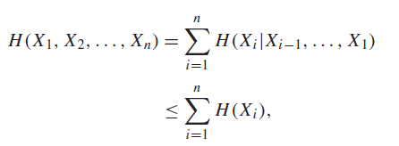
The entropy of a joint distribution just be less than the sum of the entropy of the marginals

• Proof (chain rule)

  

  The second inequality comes from the fact that conditioning reduces entropy (see conditional entropy for proof)

Which just means that independence yields the highest joint entropy.

Some properties of joint entropy

• in general, $h(x_1, …, x_n) = h(y_1, ..., y_m)$ if there exists some deterministic, injective function such that $f(x_1, …, x_n) = y_1, …, y_m$.

Conditional Entropy

The definition 🐧

We define the conditional entropy as the entropy of two random variables when conditioned on each other. This, $H(Y | X)$ gives the average entropy of $P(Y |X = x)$, so it’s basically “what’s the entropy in $Y$ that remains after I observe $X$?”

We can derive conditional entropy from the joint entropy. If $X, Y$ are not independent, then we have

The first term is just $H(X)$, but the second term is a bit foreign. This we can rewrite as

The tricky part here is that we separated out the two expectations using the probability chain rule. The inner expectation is just entropy of $P(Y | X = x)$, and we take the expectation of the entropy over $x$.

Again, from construction, if $X, Y$ are independent, then $H(Y|X) = H(Y)$, etc.

Chain rule of entropy 🚀⭐

This result is actually already obvious from how we defined conditional entropy.

This is true for any sort of further conditional, like

And this is also true for any arbitrary number of variables. Intuitively, you can just recursively collapse the variables and use the same chain rule.

Conditioning Reduces Entropy 🚀

We have $H(X | Y) \leq H(X)$, which is intuitive

• Proof (mutual information)

  We know that $I(X ; Y) = H(X) - H(X | Y)$ (see proof later down the page), and we asserted that $I(X ; Y) \geq 0$, so we are done.

Here’s a small catch: this is true on average, but it is not always true that $H(X | Y = y) \leq H(X)$. Sometimes, observation can increase uncertainty.

• Example

  Let’s say that when $y = 1$, then $x = 1$ determinstically. And when $y = 2$, then $x = 2$ with probability 0.5 and $x = 3$ with probability 0.5. Marginally, we have that $p(x = 1) = 0.98$, $p(x = 2) = 0.01, p(x = 3) = 0.01$.

  The entropy $H(X)$ is very close to 0, as we often select $x = 1$. The entropy $H(X | Y = 2)$, however, is $1$ as we select from the uniform. Therefore, $H(X | Y = 2) > H(X)$.

  Intuitively, this can happen if a rare event happens that throws off a lot of what we know, like observing a rare disease in a patient.

Some properties of conditional entropy

• $H(f(X) | Y) \leq H(X | Y)$, as with normal entropy

• $H(X | f(Y))\geq H(X | Y)$. This actually makes a ton of sense. If $f$ is injective, it’s fine. If it’s not injective, you can imagine that some of the conditioning information is lost so the entropy remaining increases

• However, $H(X | f(Y)) \leq H(X)$. You can’t make entropy increase with a conditional.

Relative Entropy 🐧

The relative entropy is intuitively a distance between distributions, which is why it’s called the KL distance.

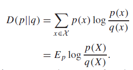
The KL distance is not a true metric. It is not symmetric, and does not follow the triangle inequality. So that’s why we also generally call $D(p || q)$ the relative entropy of p relative to q.

Generally, we assume that the domain of $q$ is larger than the domain of $p$, or else the DKL will be infinity.

A conditional relative entropy has the same idea as $H(X | Y)$, in which you sum across the condition (i.e. you take two expectations)

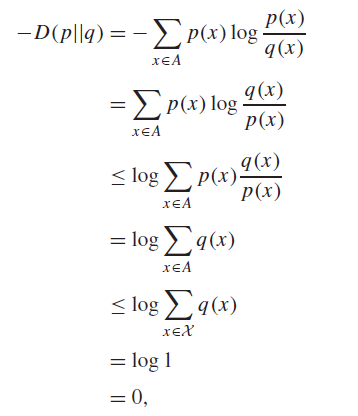
Relative entropy is non-negative 🚀

We assert that $D_{KL}(q || p) \geq 0$ with equality if and only if $q = p$

• Proof of inequality (Jensen’s + definition)

  

• Proof of forward direction (Jensen’s inequality)

  Because log is strictly concave, Jensen’s inequality says that the inequality becomes an equality when expression inside $\log$ is constant, so $q / p$ must be constant.

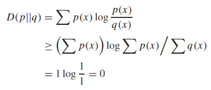
• Proof of backward direction

  $q / p = 1$, and so it’s always zero.

• Alternate proof (log-sum inequality)

  This is actually really easy. The formula is perfect

  

Relative Entropy is Convex 🚀

We assert that $D(p || q)$ is convex in $(p, q)$. In other words, if we take a linear combination of distributions, the following holds:

This does have some implications. For example, it means that KL divergence is a convex objective, which allows for convex optimization protocols.

• Proof (log-sum + definition)

  You have to apply log-sum in reverse. The LHS is already summing in the log, and so you get a less than equality

  

Chain rule of relative entropy 🚀

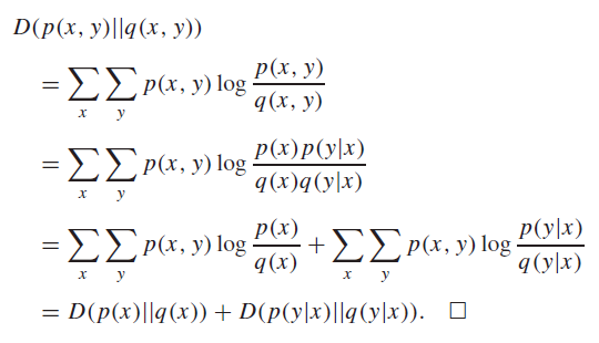
The chain rule applies for relative entropy:

• Proof (use definitions)

  

Mutual Information 🐧

We can understand the mutual information of two random variable as the following:

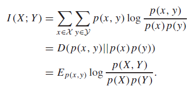
• Is $p(x)p(y)$ a true distribution?

  Yes! So this is an important concern, because KL divergences only work on true distributions. But here’s an intuitive explanation: suppose that $p(x)$ belonged to an RV $\hat{X}$ and $p(y)$ belonged to an RV $\hat{Y}$, and suppose that they were independent. Then, their joint must be $p(x)p(y)$. In reality, $X, Y$ may not be independent, but you see from this relabeling how $p(x)p(y)$ is always a valid distribtuion.

MI in terms of Entropy 🚀

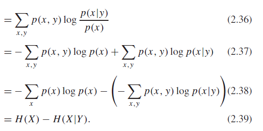
Intuitively, MI is a measure of how much information is shared between two variables. Therefore, it is only logical that this is another way to write mutual information:

The first term is how much entropy the variable naturally has, and the second term is how much entropy remains after conditioning it on the second variable. The difference is how much information is shared by X and Y.

• Proof (use KL definition)

  

  You can repeat the same derivation but factor the first step the opposite way, and yield the other definition. Therefore, MI is symmetric.

MI properties

Here are some other versions and properties of the identity

• $I(X ; Y) = H(X) + H(Y) - H(X, Y)$

• $I(X ; X) = H(X)$

• $I(X; Y) \leq I(X; Y, Z)$ (you can never lose correlation by adding more variables)

• You can’t say anything about conditioning MI, as sometimes you can increase dependency by conditioning.

• $I(X; Y | Z) = H(X | Z) - H(X | Y, Z)$ (general tip: can always tack on a conditional)
  • always a bit tricky to read: it should read [X ; Y] | Z, not X ; [Y | Z].

• $I(X;Y | Y) = H(X | Y) - H(X | Y) = 0$ (intuitively, the conditioning removes any dependence; think about graphical models!)

• Mutual information is lower bounded but is NOT upper bounded by a constant. Rather, it is upper bounded by $\max H(X), H(Y)$. Take a second to convince yourself that this is true.

• $I(f(X) ; Y) \leq I(X ; Y)$. You can show this through chain rule or $H(Y | f(X)) \geq H(Y | X)$.

Does the location of the semicolon matter?

The location of the semicolon really does matter. The expression $I(X_1, X_2 ; Y_1, Y_2)$ represents the information shared between the larger $X$ vector and the larger $Y$ vector. It could be the case that $X_1, X_2$ are highly dependent (they may be the same variable), and $Y_1, Y_2$ are highly dependent. But if all $X$ is independent from all $Y$, then $I(X_1, X_2; Y_1, Y_2) = 0$. Moving the semicolon changes which distributions you’re comparing between.

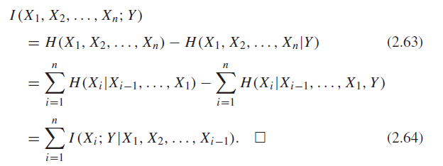
Chain rule of MI 🚀

And the general chain rule applies, which you can show through the definition of entropy

• Proof (use the entropy definition

  

Intuitively, this is just saying the shared information between the joint $X_1,…, X_n$ and $Y$.

Because MI is symmetric, we can use the chain rule on either side of the semicolon! This is because the conditional isn’t bound to one side or the other.

Note how we can “push” the Z into either side by just adding the appropriate additional information term.

MI is non-negative, and 0 if and only if independent 🚀

Both are obvious from the KL definition

Concave-Convexity of MI 🚀

This is a tad hard to follow, but if $(X, Y) = p(x)p(y | x)$, then $I(X; Y)$ is concave of $p(x)$ with $p(y|x)$ fixed, and convex of $p(y| x)$ with $p(x)$ fixed.

• Proof of first part (property of entropy)

  We know that $I(X ; Y) = H(Y) - H(Y | X)$ and we know that

  

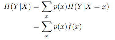
  where $f(x)$ just represents the conditional entropy. This is a dot product, which means that this is a linear function of $p(x)$.

  The first term is concave in $Y$, and because $p(y) = \sum p(y | x)p(x)$ and this is a linear function of $X$, then it is concave in $X$ too.

  Concave minus linear is still concave, as desired.

• Proof of second part (definitions of concavity)

  Imagine a mixture of conditional distributions

  

  This shouldn’t be offputting; just think of this as mixing two tables together. The joint distribution is also a mixture

  

  And so it follows that $p(y)$ is also a mixture (by marginalization)

  

  And we can create a product of marginals $q$

  

  And we know that mutual information is

  

  and we know that $D$ is convex on (p, q), which means that it is convex on the original $p(y | x)$ as well.

  ☝

  This isn’t the best of proofs. Will revisit after lecture!

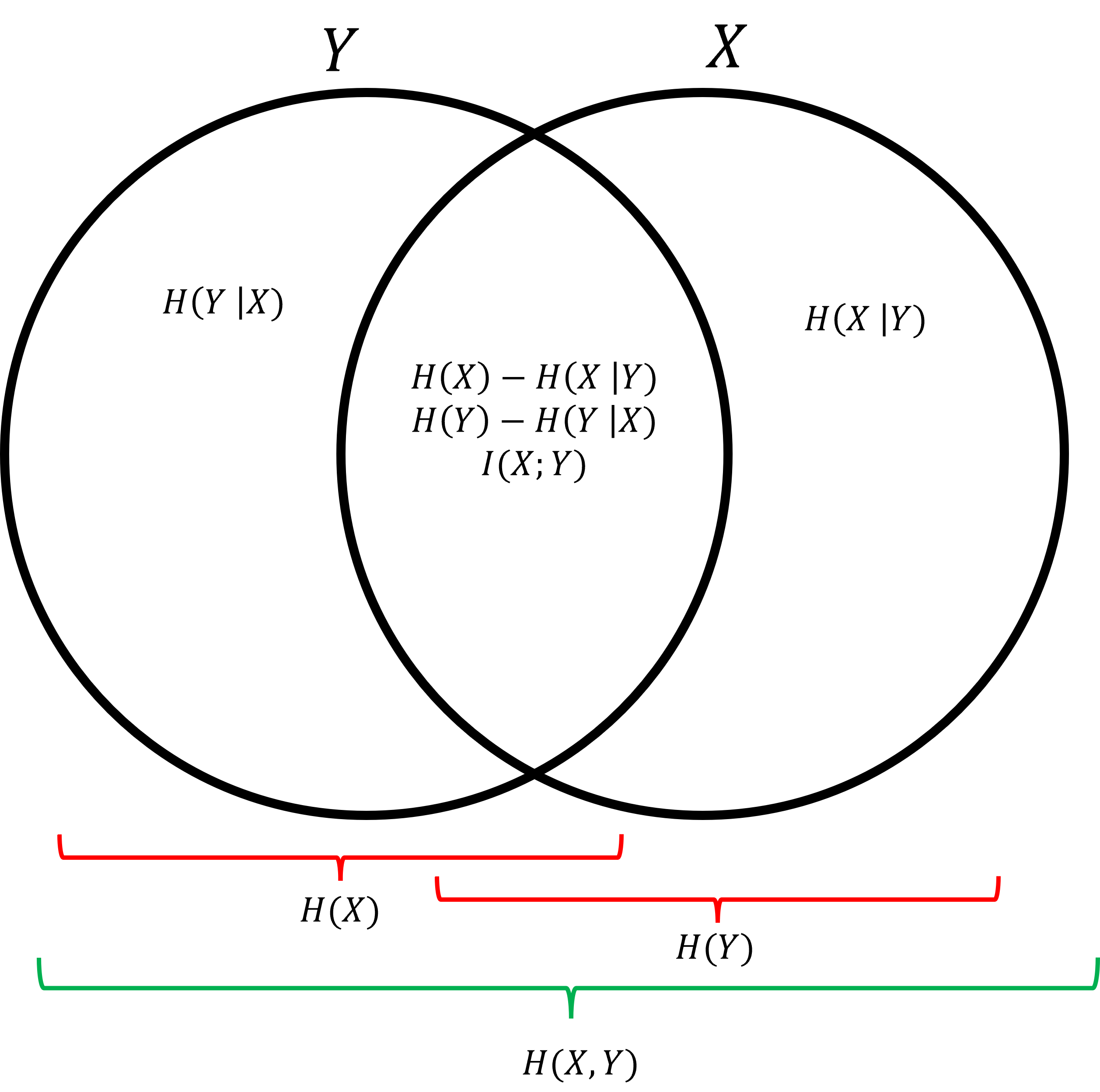
Great Diagram

This diagram sums things up. Something is “inside” a circle if it provides information. For example, if we condition on $Y$, it’s outside of $Y$ because $Y$ no longer provides surprise.

Inequalities to keep in mind

Pinsker’s Inequality

If $P, Q$ are two distributions, then

where

tl;dr the largest divergence of density is upper bounded by a quantity measurable with KL divergence.