Differential Entropy

Is there real entropy?

To establish the relationship, let’s try to quantize a continuous random variable. We can do this through a notion of riemann integrability. If we split up the distribution into sections of size $\Delta$, then the PMF of each section is

We can let $x_i$ be the center of the interval.

Let’s make a RV using this quantized version, $X^\Delta$. The entropy can be computed as follows:

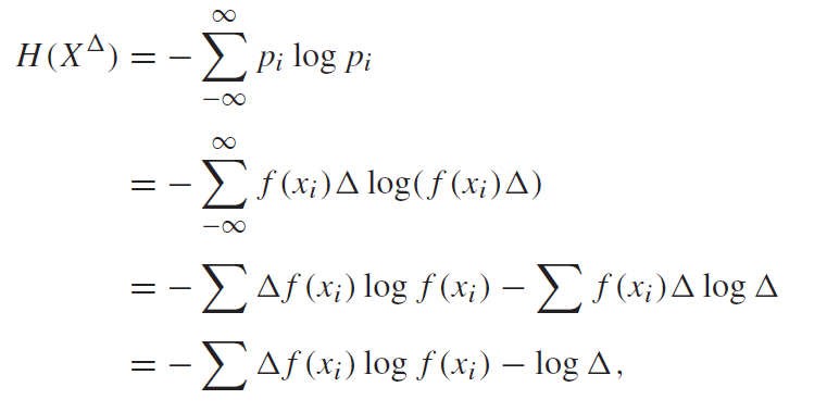
Hmmmm. So this is a problem. To get $X^\Delta$ to approach $X$, we need to have $\Delta → 0$. But as this happens, we see that $H(X^\Delta)→ \infty$. So, the entropy of a continuous random varaible is infinite.

Intuitively, this makes sense. It can take on any value; it takes an infinite number of bits to describe the variable to perfect precision.

“Fake” differential entropy

So we notice that $H(X^\Delta) \rightarrow \infty$, but we notice that it is composed of two terms: the first term is $\sum \Delta f(x_i)\log f(x_i)$, which is finite. The second term goes to infinity. But the second term is the same for all continuous RV’s, and it’s shifted vertically by this first term. So instead of figuring out the entropy, could we figure out this first term?

We define differential entropy as $\lim_{\Delta→0} f(x_i)\log f(x_i)\Delta$. If the density function is Riemann integrable, we have

This isn’t true entropy, but it has a similar form.

Important properties

Differential entropy can be negative if the interval is small enough.

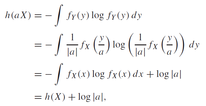
Furthermore, because scaling $aX$ means scaling the bounds (intuitively), we actually add some entropy. We get $h(aX) = h(X) + \log |a|$.

• Proof (change of variable, log properties)

  The key problem is this $1/|a|$ term. Why is this there? Well, when you’re stretching out $X$, you’re also stretching out the distribution (think of dough as it stretches thinner). It must keep its volume.

  This is fine for the linear term, but the log term doesn’t play well. This is why we are left with the extra $\log |a|$ term.

  

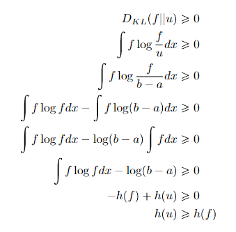
From results that you can show with KL divergence, we have $h(x) \leq h(u)$, where $u$ is the uniform. But there’s some nuance for maximizing entorpy of continuous RV’s. Stay tuned!

Results from Differential Entropy

Joint and Conditional Entropy

Joint entropy is just a multi-dimensional integral.

Conditional entropy is formulated exactly like the discrete version:

And we also know that $h(X | Y) = h(X,Y) - h(Y)$, which can be helpful. The chain rule applies for continuous spaces.

So it turns out that $h(X | Y)$ is not label invariant in $X$ as previously shown. But it is label invariant with $Y$, because $Y$ is just an outer expectation. The problem of the stretching only happens inside the logarithm.

Mutual Information

Does mutual information exist for continuous RVs? So actually, yes! We can begin with our discretized $X^\Delta, Y^\Delta$. We have

and you see how this cancels into

So this is different from the “fake” entropy. This is REAL mutual information defined in terms of the “fake” entropy.

Relative entropy

Does KL divergence exist for continuous RV’s? Well, we might start with the formulation

And you see that the $\Delta$ cancel!

Important Examples

Normal distribution

Let’s say that we have a normal distribution $\phi(x)$ with variance $\sigma^2$ and $\mu = 0$.

You can just run the derivation as follows. We will start with natural log.

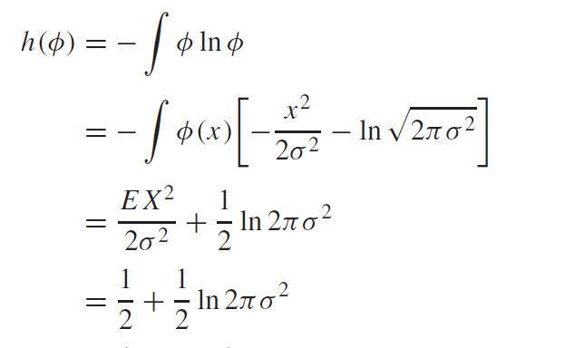
This last step is possible because $E[X] = 0$, so we can subtract $E[X]^2$ from the numerator, and this yields the variance $\sigma^2$.

And if you were to account for the extra $e$ in a base 2 logarithm, you get

which will be useful later on.

Some other interesting examples

• Because we are dealing with densities, the stretch of the distribution actually matters. For example, if $X$ is uniform on $[0, 1]$ then $h(X)=0$. Then, $H(X^\Delta) = n$, which actually makes a ton of sense (think about uniform distributions in discrete land.)

• If we are dealing with uniform on $[0, 1/8]$, then $h(X) = -3$, which means that $H(X^\Delta) = n-3$. This is intuitive, as the first three bits to the right of the deimal are 0 in all of these numbers in the interval.

• The joint entropy of a multivariate normal distribution is the following, where $|K|$ is the determinant of the covariance.

Maximizing Entropy

If you’re trying to maximize differential entropy across any support, you just make it uniform. You can prove this through the KL trick, where you do $D(p||u) = h(u) - h(p)$ in this special case of the uniform, which gets you $h(p) \leq h(u)$.

• Proof

  

With second moment constraint

But with continuous random variables, you might want to impose another constraint. Say that you wanted $E[X^2] \leq \alpha$? This is a reasonable constraint, as it’s related to variance. Essentially, you’re inquiring about how you can maximizing the entropy with a certain variance.

Well, you can do the math out (it’s very ugly), but you can show that the maximization of entropy is with a gaussian $\phi$ such that $E[\phi^2] = \alpha$. The proof is the same: you use the KL divergence.

AEP For Differential Entropy

The AEP remains mostly unchanged. We just use the notion of differential entropy instead.

Volumes

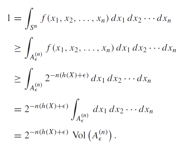
However, there does need to be a big change. Previously we talked about the cardinality; it doesn’t make sense here because we are in continuous space. Instead, we talk about the volume of the set. This is defined as

Properties of the AEP

There are exactly the same as the discrete AEP, and actually, the proofs are really the same; just replace the summation with the volume.

• Example proof of 2