Huffman Codes

The algorithm is pretty straightforward.

1. Pick the two least likely variable outcomes and make them into a leaf node. One of them gets 1, the other gets 0.

2. Combine the likelihoods of these outcomes into a super variable and add that back into the pile for consideration.

3. Keep doing this until you run out of things to code. The tree you create is the huffman tree and the coding is optimal

Deriving the Huffman code

We can make this algorithm from first principles, where we just have access to individual probabilities which we sort in order $p_1,\leq …, \leq p_m$. We know that the lengths must go the other way: $l^*_1 \geq … \geq l^*_m$. Otherwise, you can just swap two lengths and we will get a shorter expected code length.

Furthermore, as we will be dealing with binary codes, we know that $l^*_{m-1} = l^*_m$. If this isn’t the case, say $l_m = l_{m-1}+1$, then we know that $l_m$ doesn’t have a sibling, which means that it can be “rotated” to form a shorter tree.

Finally, we know that $\sum 2^{-l_i} = 1$ (again, because this is binary). So it makes sense to start thinking recursively. We can make $l_{m-1}$ and $l_m$ share a common parent node. This parent node has length $\hat{l}_{m+1}$. We dopn’t know these numbers yet, but we can rewrit4e our objective:

which we can refactor into

and this just looks like the old form with one fewer term! (because the term outside of the parenthesis doesn’t matter)

The constraint is

which again collapses down into the familiar form.

Huffman code analysis

The complexity of the Huffman code is wholly the sorting operation which takes place after every run. It takes $n\log n$ to sort initially, and $\log n$ to insert the new value. So, overall it’s $O(n\log n)$, where $n$ is the size of the alphabet.

Ultimately, Huffman does a good job, but it’s not using a lot of information. It only uses the distribution of each character and encodes it separately. Longer sequences might have better structures to exploit, but because of the complexity depending on the alphabet size, we can’t just “chunk” together RV’s to form an alphabet $\chi^n$ size (or else we risk blowing up the complexity).

Arithmetic Codes

Huffman codes are elegant, but they aren’t good at encoding long sequences (i.e. it makes the inductive assumption that everything is IID, and will encode single characters. Arithmetic codes are designed to encode long sequences with linear complexity, although the range of encoding is more limited.

The tl;dr is that arithmetic codes turn the code into binary decimal representation, which yields some very nice properties

Arithmetic Code setup

Let’s suppose that you had IID $X_1,…,X_n$ that are sampled from some alphabet with size $|\chi|$. Your goal is to encode them into $U_1,…$ as optimally as possible. This means that the $U_1,…$ must be distributed uniformly (or else we can run $U_1,…$ through the encoder again and get something even better, etc.

The goal of an arithmetic code is to find a function $F$ that maps between $X_1,.., X_n$ (multinomial distribution) to a uniform distribution.

Binary Decimal Representation

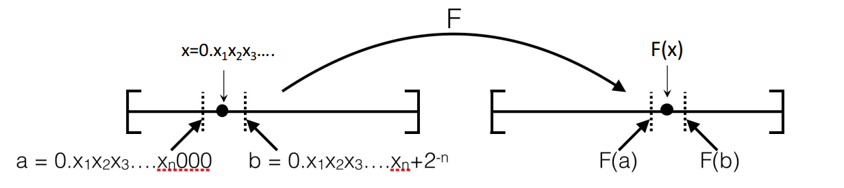
The trick here is to turn the list of RV’s into numbers. How? Well, we can consider binary decimals: $X_\infty = 0.X_1,…,X_n...$ and $U_\infty = 0.U_1,…$ We assume that these are infinite-precision decimals (and we’ll explain why).

The $X_\infty = 0.X_1,…,X_n$ is some sort of distribution expressed in base $|\chi|$.

The $U_\infty = 0.U_1,…$ is a uniform distribution, because every $U$ is taken uniformly for maximal entropy.

Why do we use this setup? Well, there are a few nice properties

• It is possible to create an invertible mapping (see below)

• when you add more data, like $X_{n+1}$, it doesn’t require you to recompute any of the previously sent bits; adding more data to the beginning just means adding more data to the end.
  • why? Well, when you have $0.X_1,…,X_n$, you are bounding the outcome between $0.X_1,…,X_n$ and $0.X_1,…,X_n + |X|^{-n}$ (think about it: we are asuming an infinite decimal). Adding another decimal place will only shorten this bound.

• the CDF can be computed recursively (see below)

The Mapping Function

So you just need to find some function $g$ that maps the $X$ binary-decimal representation to the $U$ binary decimal representation. To do this, we start with the simplest constraint: $p(g(x)\leq u) = u$. This is only true for uniform distributions. This yields $p(x < g^{-1}(u)) = u$, and we know that the left hand side is just $F$, the CDF. So we have

and a natural choice for $g$ is

Is this well-defined? Well, we know that $F$ is monotonically increasing. We also know that every possible sequence of characters have a non-zero probability, which means that $F$ is always increasing and therefore invertible. And we showed int he last section that this $F$ has some really nice properties that make it easy to compute

Computing the Mapping Function (CDF)

We can compute the cumulative function recursively

The first term you have by previously getting $F$, and the second term is just a CDF function of $X$. The second term can often be factored by the probability structure and computed directly.

For the upper bound, we realize that $F(0.x_1,…,x_n,111111…)$ is just a marginalization across all $X_{n+1}…$, which is equivalent to doing $F(0.x_1,…,x_n)+p(x_1,…,x_n)$.

The actual coding

The actual coding is surprisingly easy.

1. Turn any sequence $x_1,…,x_n$ into a number $0.x_1,…,x_n$ (expressed in base $|X|$).

2. Create lower bounds $a_n = 0.x_1,…,x_n$$a^n = 0.x_1,…,x_n$ and upper bounds $b_n = 0.x_1,…,x_n + |X|^{-n}$

3. Recursively compute $A_n = F(a_n)$ and $B_n = F(b_n)$ using our CDF formula

4. On the new number line in $U$ space, consider $[A_n, B_n]$. Take the middle of the bounds, and use the entropy limit $\lceil \log 1/p\rceil$ to decide the number of decimal places to send
   1. The middle of the bounds is arbitrary. Any number inside these bounds will map to the right number in the $X$ space.

The actual decoding

So this is pretty interesting. Here’s something interesting. When you’re dealing with an unknown bit, you can split it into two intervals: $[0.x_1,…x_n0, 0.x_1,…x_n01111…]$ and $[0.x_1,…x_n1, 0.x_1,…x_n11111…]$. If you compute this, it’s a clean split. But if you’re in one interval, you know what the next bit will be!

The second realization is that these intervals map very cleanly into the $U$ space. You should convince yourself that it maps the clean 50/50 split into a (1-p) / p split. This makes sense, actually. The algorithm is therefore

1. Split the intervals

2. map the intervals to U space

3. look at your current $U$ expansion $0.u_1,…,u_m$. This forms an interval $[0.u_1,…,u_m, 0.u_1,…,u_m11111…]$. If this interval is firmly in one of the intervals created in step 2, then you know what bit should go next in the data. Else, add more $u$ until we are firmly in an interval.

4. Rinse, repeat.

Lempel-Ziv Coding

The idea is actually stupidly simple. Given a string, find out how to express the next characters using a substring that has been previously expressed.

Sliding Window LZ Algorithm

If $W$ is your window size and you’ve compressed up to $i-1$, then the next compression move is to find some $i-1-W \leq j \leq i -1$ such that $x_{j+l} = x_{i+l}$ for all $l<k$, where $k$ is the largest possible. You denote this compression with two possible tuples: $(F, P, L)$ is when you specify the start point $P$ and the length of the match $L$. $(F, C)$ is when you can’t find anything and need to specify an uncompressed character (usually close to the beginning). The $F$ is a flag bit that tells us what type of tuple we’re looking for.

Concretely, this is the algorithm

1. Start with a sliding window $W$ that looks backward

2. For the current position, see if you can find a non-trivial substring in the previous window. If you can, mark where it starts and the length $k$
   1. if you can’t, just encode one character

3. Slide the window forward $k$ steps until the previously encoded string is now in the window

To decode, you just construct the code. Because the code will only depend on things in the past, it is trivial to construct

Proof of optimality

Here’s the general sketch: as $n→\infty$ (the size of the coding chunk) as long as the window $W$ stays large enough, the probability of including a typical set in $W$ approaches 1. Why is this important? Well, it just means that we are arbitrarily likely to find what we need in $W$.

• The proof

  First: we bound the probability of some typical sequence not happening in W

  

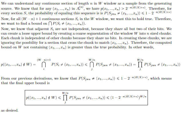
  Next: we use a union bound on the probability of at least one element in typical set not appearing

  

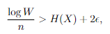
  Next, we establish the following relationship between $W$ and $n$:

  

  And you can show that the probability of at least one element not appearing will pinch to 0 (this is an algebraic slog, so I omitted it).

  Finally, we can see two properties

  1. $\log W / n$ is the average bits per message character, and we know that this gets close to $H(X)$. This shows the optimality. Why? Well, $\log W$ is needed to specify the location of the found string in the window.

  2. We don’t need to worry about the length of the code $n$, because you need $\log n$ bits for that, and $\log n / n → 0$.

Tree-Structured LZ Algorithm

We parse the source sequence into the shortest strings that have not appeared so far. So this means that you’ll be building up longer and longer strings. And more specifically, for every element in this sequence, its prefixes must have all occurred earlier. More specifically, if you cut off the last character of the string, this shortened string must have occurred before, or else we wouldn’t have encountered this current element.

Therefore, we can send the parsed strings by giving the location of the prefix and the value of the last symbol. More on this later

Which coding algorithm should I use?

When coding, you need to consider three potentially relevant steps

1. Learn statistics of the coding data

2. Construct code

3. Use the code to encode the data

So let’s compare the three previous methods

• Huffman code is a very elegant approach, but it requires all three steps and is exponential in the number of bits to encode (we need multiple bit encoding, as often the closeness to optimality is asymptotic in bit length).

• Arithmetic code skips step 2, and can construct the code using only the statistics. It is also linear in the bit length

• Lempel-Ziv skips steps 1 and 2 and encodes directly from the data

All are asymptotically optimal.