Proof tips

• typical sequences is bounded individually in probability. We also know that probabilities are bounded in summation, so we can use these two bounds to our advantage

• Notation: $Pr(B)$ or $Pr(A)$ means $\sum_{x\in A} p(x)$, etc.

Sending Codes

So let’s formalize the problem of code-sending and establish why we care. You want to send a message that you don’t know (not pre-determined) across a channel. For now, let’s assume that the channel has no noise. Can we send with as little number of bits as possible?

We model the code as a string of random variables. The parameters of the random variables are determined by the source (think of each random variable as a character, etc). Depending on the properties of the random variable string, you may find some neat properties.

In reality, the RV’s are dependent on each other through the markov property with potentially a long history (think natural language). However, we may, as a simplification, think of them as IID. This section shows some critical theory under this IID assumption. How can you best compress a string of samples?

AEP Theorem 🚀

It is similar to the law of large numbers. The law of large numbers says that the average of samples is close to the expectation of an RV. The AEP states that you can approximate the $H(X)$ by taking samples $X_1, … X_n$ and computing $\frac{1}{n}\log \frac{1}{p(X_1, …, X_n)}$.

Formally, if we have IID $X_1, … X_n$ from some distribution $p(X = x)$, then

Or, more formally, for every $\delta$, there exists some $N(\delta)$ such that for all $n > N(\delta)$, we have

You can understand that this $\frac{1}{p(X_n)}$ is a random variable where you sample something and feed that right back into its own distribution. So it follows from the law of large numbers that the AEP is true.

Generalized AEP

We will talk about entropy rates later, but you can essentially say the same thing about $H(\chi)$, where $H(\chi)$ is the entropy rate. In other words:

Understanding AEP

To truly understand the AEP, let’s look at an example with bernoulli with probability $p$. In this IID sequence, permutation doesn’t matter. It only matters the number $k$ of ones in the sequence. Recall that $p(x^n) = p^k(1-p)^{n-k}$.

Now, if you plug this into the AEP, you can say that

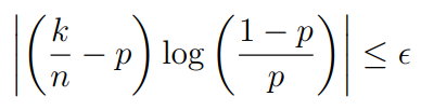
which is equivalent to

which should remind you a lot of the law of large numbers. Just set $\epsilon’ = \frac{1}{\log(1-p)/p}$ and you’re done. This gets you a bound $|k/n - p| \leq \epsilon’$ for every sequence of $k$ terms that are in the AEP. Because the AEP has $Pr(A) \geq 1-\delta$, it means that for any $\epsilon’$, we can show that any sampled sequence has $k/n - p$ is within an epsilon sphere with confidence $1-\delta$

When does this break down? It breaks down when $p=1/2$ and $\log(1-p)/p = 0$. In this case, there is no bound on $k$. This makes sense as the probability no longer depends on $k$ if $p = 1/2$.

Typical Sets 🐧

We define the typical set $A_\epsilon^{(n)}$ as the set of sequences $(x_1, x_2, …, x_n)$ drawn IID from $X$, where

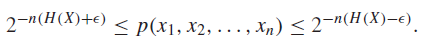
Don’t try to think about why these bounds exist; as we will see, they exist only so we have some nice properties.

Intuitively, the typical set is just the set of sequences that are the least surprising. A typical set may be a small subset of all set of sequences, but as we will see below, an element sampled from the random variable is highly likely to be one of the typical set elements.

As a non-probability version equivalent, you might consider the set of samples whose mean is within an epsilon-ball of the true mean. This is a typical set for estimating sample means. If you’re ever confused, think of means instead of entropy, and all of the properties should be intuitive.

Properties of Typical Sets

1. For all sequences inside a typical set, we have $H(X) - \epsilon \leq \frac{1}{n}\log \frac{1}{p(x_1, …, x_n)} \leq H(X) + \epsilon$. for any $\epsilon > 0$ and large enough $n$. In other words, inside the typical set, our estimated entropy is within an epsilon-ball of the true entropy. Proof through Typical Sets definition.

2. The probability that a sequence belongs in the Typical Set approaches 1: $P((x,…) \in A_\epsilon^{(n)}) > 1 - \epsilon$ for a sufficiently large $n$.
   • Proof (Using AEP)

     By the delta-epsilon definition of AEP, we have that

     

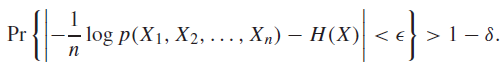
     which is true for all sequences of random variables. Now, we observe that when this log-prob is inside the epsilon ball of $H$, it ALSO corresponds to being in the typical set. Therefore, we just need to set $\delta = \epsilon$ and we are done.

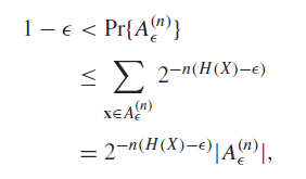
3. There is an upper bound to the number of elements in the typical set: $|A_\epsilon^{(n)}|\leq 2^{n(H(X) + \epsilon)}$.
   • Proof (definitions)

     This should be pretty obvious. The probabilities of each element in the typical set is upper bounded

     

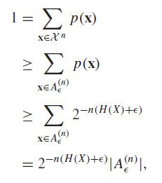
     which you can easily solve.

4. There is a lower bound to the number of elements in the typical set: $|A_\epsilon^{(n)}| \geq (1-\epsilon)2^{n(H(X)-\epsilon)}$.
   • Proof (using property #2)

     

The variance in probability increases with $n$ due to the $n\epsilon$ term. This is actually pretty intersting!

Data Compression with AEP

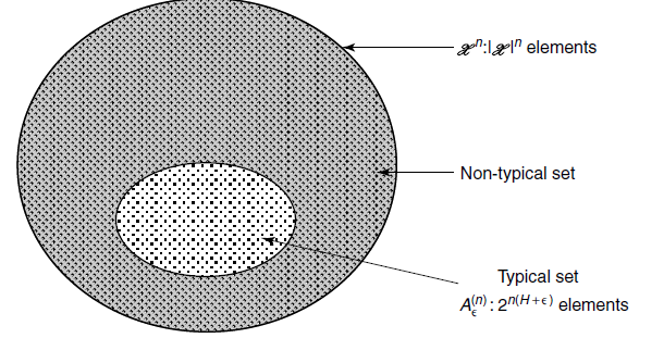
So here’s the big point of talking about AEP. It seems weird to be able to compress things of size $|X|^n$ into their entropy $nH$ on expectation, because it feels like we are shoving too much data in too little space. Information theory focuses on how compression is possible. By showing that a Typical Set expands to become $\epsilon$-close to the full probability mass, and by the knowledge that the Typical set is bounded by size, then we know for certain that we can indeed encode with $H$ bits per character.

Naive Compression

Naive compression assigns an index to every possible sequence, which has size $|\chi|^n$. We can rewrite this as $2^{n\log |\chi|}$, which means that it takes $\log |\chi|$ bits per sample. Can we do better?

Using Typical Sets

Because there are at most $2^{n(H + \epsilon)}$ elements in the typical set, we can describe it with $n(H + \epsilon)$ bits, which means that we only use $H$ bits per sample.

Now, interestingly, if the distribution of $X$ is uniform, then $H(X) = \log |\chi|$, so the typical set is everything, and all encoding is equally inefficient. So this establishes, through theory, what we mean by compression.

Optimal Coding theorem 🚀

Let $X^n$ represent an n-length sequence. There exists an invertible code such that

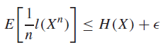
• Proof (properties of Typical Set)

  The key insight is that with large enough $n$, the probability of being in the Typical Set is $1 - \epsilon$ for any $\epsilon > 0$. We can set up the derivation like so

  

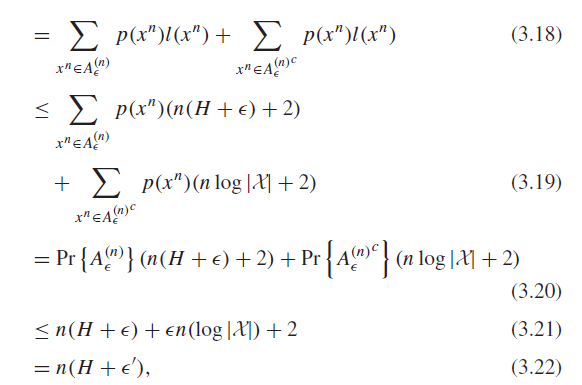
  And this is sufficient (just let the original $\epsilon$ be such that $\epsilon’$ is the $\epsilon$ in the theorem (classic analysis trick)

So the tl;dr is that on average, we can represent sequences $X^n$ with $nH(X)$ bits on average! But how can we actually do this? Well, we’ll find out the concrete coding schemes in the next set of notes.

Ultimately, why shall we care?

We have established a theoretical possibility of coding. And in fact, we can technically have a primitive proof-of-concept code in which we assign a code of length $H$ to sequences inside the typical set, and kept all other sequences as-is. In this case, we have shown that the compression length is $H(X)$ asymptotically.

But this is super primitive and has problems.

In later sections, we will show how prefix codes can reach this theoretical possibility, to within one bit.

High Probability Sets

We define a high probability set as $B_\delta^{(n)}$ as the set such that $P(B_\delta^{(n)})\geq 1-\delta$. In other words, the probability of being in this set is larger than $1-\delta$.

We can construct $B$ greedily by taking the most likely sequences first. As it turns out, $B^{(n)}$ has at least $2^{nH}$ elements, which is in an order of exponent of $2^{n (H \pm \epsilon)}$, which is the size of $A^{(n)}$.

The takeaway is that the highest likelihood sequences (high probability sets) have intersections with the typical set.

High Probability vs Typical sets

The tl;dr is that B is limited as a set (to the likelihood), while A is limited per value (by being within the right range). You can’t say much about $B$, but $B$ is related to $A$ through some simple properties.

The high probability set is subtly different from a typical set. If we construct the smallest possible high probability set in a bernoulli sequence with $p = 0.8$, you will definitely see the sequence where everything is 1. However, the typical set may not contain that. The typical set contains samples whose probabilities are closest to the empirical entropy, which may not include the highest possible likelihood (because that may not be surprising enough!)

However, we do know from basic probability that for $P(B_\delta^{(n)})\geq 1-\delta$ and $P(A_\epsilon)\geq 1 - \epsilon$ (true for large enough numbers), we have

which means that there is a large intersection between the high probability and typical sets.

We also know that the smallest possible $B_\delta$ is upper bounded by the size of $A_\epsilon$ at large enough $n$, as the $A$ set gets close to the full set, while the smallest possible $B_\delta$ is upper bounded by $\delta * |\chi^n|$.