The idea

Some distributions are better explained with a latent variable, such that $p(x | z)$ is easier to model than $p(x)$.

The simple model

Mixture of gaussians is a very simple latent model where $p(x | z) \sim N(\mu_z, \sigma_z)$ and $z \in Cat(k)$. We know from 229 that we can apply EM algorithm to iteratively cluster the data and perform maximum likelihood. We need to create a posterior $p(z_i | x)$, which is possible because $z$ is categorical.

VAE is an infinite mixture of gaussians

Because every $z$ defines a unique gaussian, the marginal $p(x)$ can be interpreted as a mixture of an uncountably infinite number of gaussians, which is why $p(x)$ is so expressive.

Moving to Variational Inference

In our derivation today, we are taking inspiration from EM but we are doing it in a more sophisticated way. Or, rather, we are forced to do it differently because we are now defining $z$ as a continuous random variable.

There is a big pro to this: the marginal $p(x)$ becomes really complex and flexible because it’s a mixture of an infinite number of gaussians!

Moving towards the Lower Bound

Attempt 1: Naive Monte Carlo

The idea here is that we can approximate the marginalization by doing

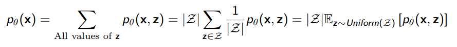
by definition of expectation, which means that our Monte Carlo estimate would be

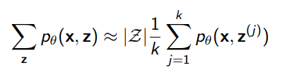
However, because we are in such a large sample space, the true $p_\theta(x, z)$ is very low, which means that this is very high variance. You may never “hit” the right completions.

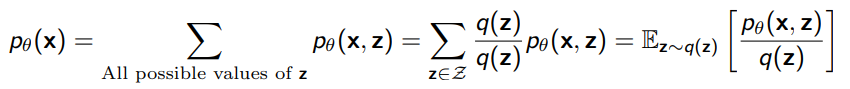
Attempt 2: Importance Sampling

If we had a surrogate distribution $q(z)$, we could rewrite the problem as

And we could approximate with sample average

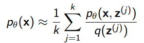
Because of the linearity of expectation, it’s trivial to show that this is an unbiased estimator of p(x).

Adding the Log (and deriving ELBO)

Because we want the log-likelihood, we take the log of the whole empirical expectation

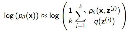
Now this is not necessarily the best expression to follow, but Jensen’s inequality states that this is a lower bound to

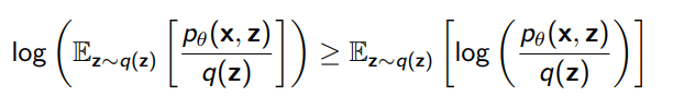
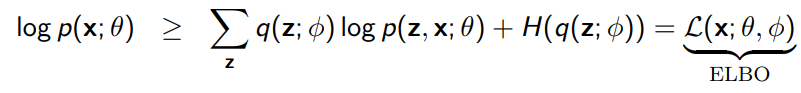
Which we call the Evidence Lower Bound (ELBO)

We can split this quantity up into

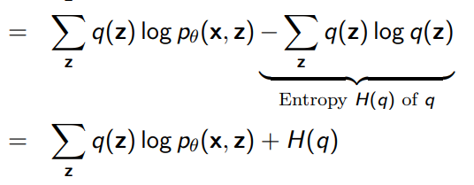
And we can show that the equality holds if $q = p(z | x)$.

Tightness of ELBO bound

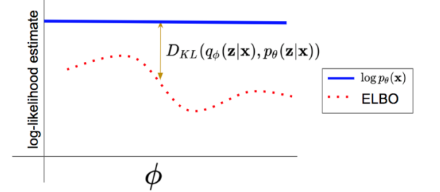
The tightness of the bound we can also determine! If we ditch the Jensen’s inequality and move backwards from the KL divergence between $q(z)$ and $p(z| x)$, we get

From RHS we can reassemble the ELBO, but because we have an equality, we can say that the bound gets tighter with $D_{KL}(q || p(z|x))$. Or, in other words:

This is a nice diagram

How do we actually train?

So recall that

How do you actually optimize for $\theta, \phi$?

Variational Learning

Two facts:

1. We can increase $\mathcal{L}$ by optimizing over $\theta$. Note that this ELBO holds for any $\phi$, which means that if we optimize for $\theta$ at any time, we’re doing something about the lower bound

2. Note that we can also increase $\mathcal{L}$ by optimizing over $\phi$.

Concretely, this means that you perform alternative optimization on $\phi$ and $\theta$, much like in the EM algorithm!

The key difference from the EM algorithm is that we’re not fitting $\phi$ towards the posterior explicitly. However, implicitly, by increasing the $\mathcal{L}$ without changing $\theta$, we’re tightening the bound. Think about this for a second. The left hand side, $p(x ; \theta)$ is only dependent on $\theta$. So, if you optimize over $\phi$ and $\mathcal{L}$ increases, the only way this happens is if the KL term goes down! So you’re performing the E step implicitly.

Computing Gradients

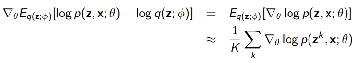
The gradient respect to $\theta$ is easy:

But what about $\phi$? How do we optimize through the expectation?

Idea 1: use Monte Carlo sampling:

This works because you’ve actually nullified the gradient in the expectation sample. This is OK, but we can do better. We can improve using REINFORCE (policy gradient), but for now, there’s a cheap trick called the reparameterization trick when your distribution can be split into an affine sum of means and scaled variances.

If $q(z;\phi)\sim N(\mu_\phi, \sigma_\phi^2)$, then $z\sim q$ is the same as $z = u + \sigma \epsilon, \epsilon \sim N(0, 1)$. Note: it’s not $\sigma^2$, it’s $\sigma$ that you scale $\epsilon$ by. This is important because you’ve booted the parameters out of the distribution! This gets you

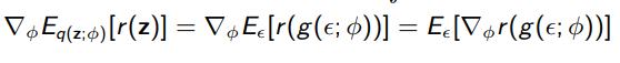
Which is computable through Monte Carlo estimation. This is far lower variance than the unscaled version, and it preserves parameter dependence!

Amortized Inference

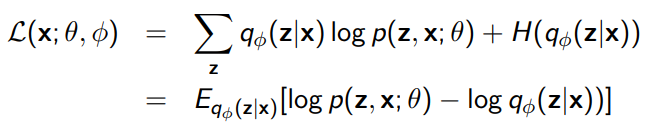
The idea here is to generalize $q(z;\phi)$ to one neural network for all datapoints, $q(z|x; \phi)$. Everything else stays the same and you get ELBO

Perspective as autoencoder

If you play with the ELBO and do some rearrangement, you will get this:

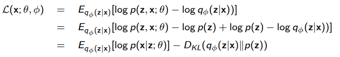
The $q$ is your encoder. You can take some input and map it to a latent space $q_\phi(z|x’)$.

The $p$ is your decoder. Sample any $z$ and you can get $p(x | z)$.

The first term in the rearrangement of the ELBO is the reconstruction objective. The second term is a regularization objective. What is $p(z)$? Well, it’s some prior. We can assume that this prior is a simple distribution, like a gaussian. We constrain the output distribution of $q(z|x)$ to be close to the prior $p(z)$.

This prior doesn’t get drawn out of thin air; when you compute $p(z, x)$ in the original setup, you need to factor as $p(x | z)p(z)$, and here is where your prior comes in.

We call this KL term the variational bottleneck

Regularization and Posterior Collapse

So you might be wondering: if we’re constraining $q$ to be close to the prior $p$, wouldn’t that destroy the purpose of $q$? Yes! But $\mathcal{L}$ can be maximized without this KL being zero, because this $q$ modifies the first term too. In fact, in an ideal system, you want $q$ to not be the same as $p$.

If $q$ approaches $p$, this is known as posterior collapse, and it means that the intput is no longer giving information to the latent space.