Score-Based Models

Tags	CS 236

Moving to score models

Previously, we dealt with representations of $p(x)$ either explicitly (through parameterized distributions) or implicitly (through energy models).

Pro: we can train with maximum likelihood and we can potentially compare models through likelihoods, etc.

Cons: partition functions are intractable and more generally, marginalizing latents are intractable, leading to the need for surrogate objectives.

Previously, we also dealt with sampling-based models, like GANS, where we defined a way of sampling from the desired distribution

Pro: samples can be higher quality

Con: unstable, hard to compare or gauge progress or training

Score Functions

The score function ( $\nabla_x \log p(x)$ ) is a really nice choice that removes some of the cons of the probability parameterization while keeping a degree of stability. Intuitively, because we are dealing with gradients, we don’t care about any constant offset (partition function)

All distributions have a vector field, although not all vector fields correspond to valid distributions. Particularly, many vector fields are not conservative, which means that it doens’t correspond to a distribution. We can choose to ignore this, which removes a constraint, and it allows for easier optimization.

In general, score functions are simpler to represent than the density.

Score Matching

The difficulty: we take some $p_{data}$ , get samples $x_1, …, x_n$ . How do we estimate a score function $s_\theta(x) \approx \nabla_x \log p_{data}(x)$ ?

If you visualize the scores as vectors, you can try to regress the vectors to the true data

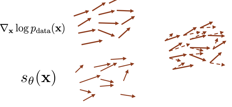
If you formalize this difference as squared L2 distance, you get the Fisher Divergence objective

And from our discussion in EBMs, we know that this objective is the same as the following:

Which is optimizable without knowing the true score function. The caveat is that the score model needs to be simple to evaluate—and even the jacobian.

Unfortunately, this is not scalable. To get the diagonal of the jacobian, we need to do $n$ backprops through the model, one for every gradient. There isn’t a parallizable operation that can be done.

Sliced Score Matching

We can reduce the complexity by looking at squared distance of the projection of the scores

and in a similar way, we can show that this becomes

This is a big improvement in efficiency, because the inner product of the jacobian is computable in one backwards pass. This is true because we can rearrange the elements as

And you can imagine adding a last layer onto the score network that computes $v^Ts_\theta(x)$ . The gradient pass is exactly $\nabla_x v^Ts_\theta(x)$ .

You can do this multiple times with random projections to get an estimate of the score matching objective.

In reality, these methods are comparable to non-sliced score matching while being much, much lower in complexity.

Denoising Score Matching

In the previous section, we found one way to estimate the score. In this section, we will take a very different way of estimating the score of a noised input. This has a clean formula, and from Tweedie’s formula, we can use the noised score to denoise something.

The Setup

If we perturb the data distribution by adding gaussian noise, we assert that we can do a special trick. The perturbation is defined as

And visually, it just “fuzzies” up the data. We assert that we can estimate

\nabla_{\tilde{x}}\log q_\sigma(\tilde{x})

Estimating the noisy score

We start by asserting that the score matching objective

is the same (up to a constant that doesn’t depend on $\theta$ ) as the following:

Derivation (definitions, log-gradient trick)
To show this, let’s first expand out the score matching objective
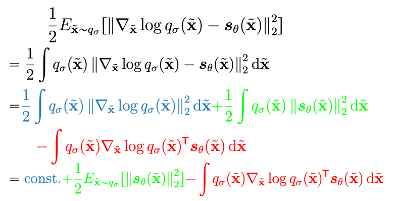
Now, let’s focus on the red part. We can use a simple combination of tricks and definitions to manipulate the expression into
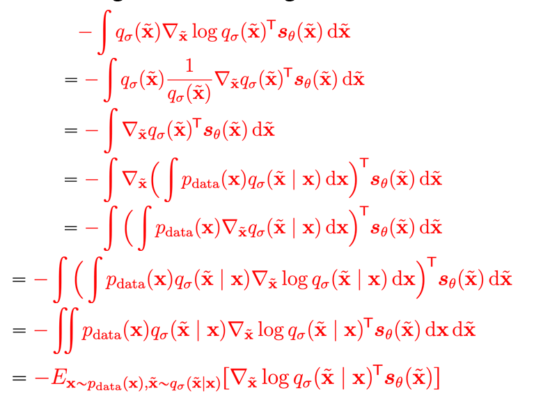
Now, let’s plug everything back in. The score matching objective is the same as:
which from above becomes
Using inner product properties, we get
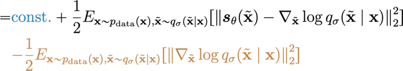
and the brown part is a constant. So, we get the final objective

Now, this is a key insight because the distribution $x, \tilde{x}$ are easy to sample from. Furthermore, the gradient of the conditional distribution is easy to compute (in fact, it’s closed form)

The upshot is that we can therefore create a score model that estimates the score for the noised data distribution using samples from the clean distribution.

So concretely, to train noisy score

Sample datapoints

Sample noisy datapoints

Regress using the derived objective using Monte Carlo estimation of the objective

Noisy Score as Denoising

If we express the noisy score objective with a gaussian, it reduces into

of if you choose a unit gaussian, we have

which means that the objective becomes estimating the noise added to the model! Keep this in mind for later.

We can show this the other way around using Tweedie's formula. So if we think about denoising some $x$ from $\tilde{x}$ , we want to compute

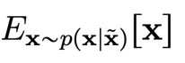
Now, Tweedie's formula states the the following is true about expectations of posteriors:

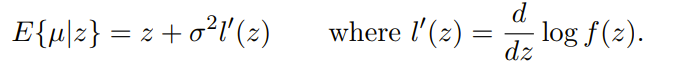
As long as $z\sim(\mu,\sigma^2)$ . This gives us a very nice formula for the denoising objective!

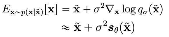
As such, we have shown in two directions that estimating noisy score is the same thing as estimating a denoising objective.

What’s wrong with Noisy Score?

Our final objective is to find the distrubiton of $p(x)$ , but we’ve created the score function to the noised distribution. As such, we can’t directly apply the noisy score to get our $p(x)$ . Furthermore, we can’t let $\sigma$ go to zero, because the variance of the score actually explodes (due to the $\sigma^2$ term in the denominator.

As we will see in later sections, we can use noisy score as an iterative process, which yields diffusion models. For now, just know that we can use samples from the dataset and noise perturbations to estimate the score of the noised dataset.

From Scores to Samples: Initial Approach

If you have a score function $s_\theta(x) = \nabla \log p(x)$ …how do you sample from $p(x)$ ?

Naive approach: follow scores

The idea here is simple. If it’s just the gradient of likelihood, why not perform gradient ascent?

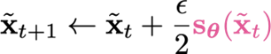
This is a good start, and this will get you $x$ that is the mode of $p(x)$ (maximizing the likelihood). However, this is not what you want. You want a sample from $p(x)$ .

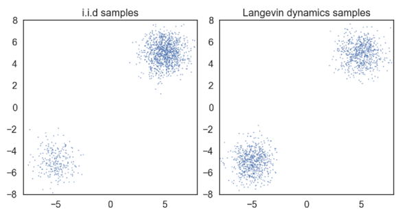
Langevin MCMC

You can prove this formally, but if you model the $x_t$ as a stochastic MDP, if you inject some noise into the ascent process, you will get a sample from $p(x)$

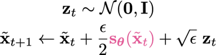
Asymptotically, as $\epsilon → 0, T → \infty$ , $x_t \sim p(x)$ .

Concretely, you

Start from noise

Run this Markov Chain until convergence

The samples you get from the Markov chain are samples from $p(x)$

What’s wrong?

So in theory, Langevin MCMC has a staionary point of $p(x)$ , so if you had a perfect estimate of the score function, you could start $x$ from noise and get the correct distribution after annealing.

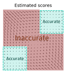
The main problem is that the estimation of the score function isn’t perfect. The data points could lie on a thin manifold in the true output support.

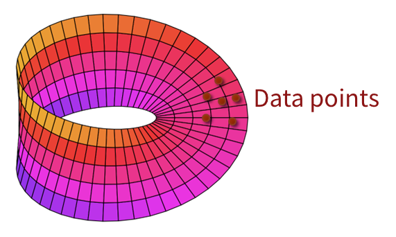
Indeed, you can reduce the data dimensionality significantly and get a very similar reconstruction, which indicates there does exist such a manifold. This is a problem for two reasons. First, it means that everything out of the manifold is OOD (including the noisy image intermediates). Second, it means that the score itself becomes undefined, or at least not very tame, as we approach these manifolds.

The OOD is a larger problem, because, again, we start on these OOD samples. So the estimate of the scores are wildly wrong, which means that we may never get to these accurate, in-distribution regions

A side problem: Langevin dynamics doesn’t play well with different data modes, i.e. it will find the modes but because we are dealing with log likelihoods, we end up ditching leading constants. Therefore, a multimodal distribution is recreated without any emphasis on the weighting on the different modes. This could lead to the score function amplifying a rare mode as much as a common mode, leading to sampling problems.