Diffusion Models

In this next section, we will solve the problems established above, which moves us to diffusion models.

Gaussian Perturbation

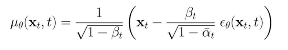
Here’s the insight: our model doesn’t fit well because the samples are in a manifold, and everything else is OOD. Now, what if we “fattened” the manifold by adding gaussian noise? After doing this, it’s no longer a manifold anymore.

Adding noise is a surefire way of increasing the space that the samples take up. For instance, you can imagine adding so much noise that the original data is lost to the noise.

• Pro: you’re increasing the size of the reliable data support, which means that the Lagenvin dynamics are more useful.

• Con: the more noise you add, the further away the data becomes. In other words, when you estimate a score for this data, it may be different from the score of the unnoised data

We estimate these noised scores using our noisy score matching paradigm (very convenient!)

• Good diagram

  

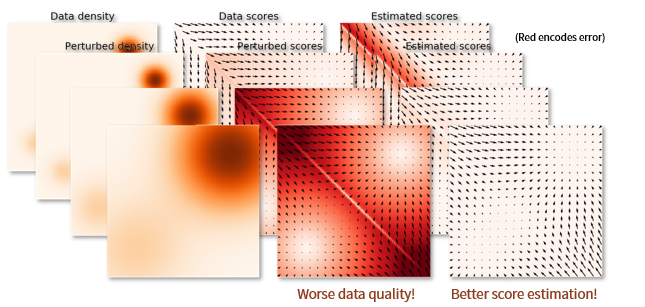
  As you add more noise, the score estimation of the noised distribution becomes better because the distribution is wider. However, the true scores of the noised distribution becomes further away from the true score of the original distribution. So, it’s an unfortunate tradeoff.

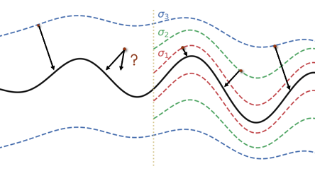
Using Multiple Noise Scales (Noise Scheduling)

Here’s the idea: can we somehow anneal the noise? When you start, you are at a very high noise level, and it’s easier for you to fit a highly-noised version of the data. Then, as you get closer to that distribution, you can change the objective to fit a lower-noised version, and so on and so forth.

By adding these degrees of noise, you’re making it much easier to approach the mode of the distribution by allowing the score function to be more accurate throughout the process

• Example of this process

  

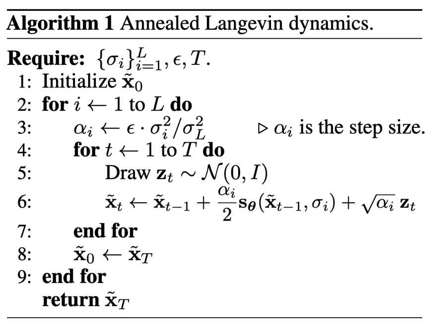
This process yields the Annealed Langevin Dynamics paradigm

• Algorithm

  

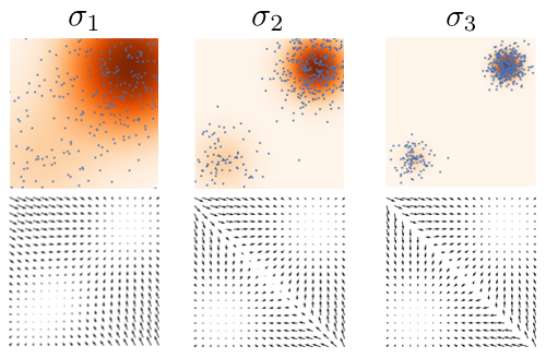
Noise Conditioned Score Networks

This means that you have to specify a $\sigma_i$ into the score function, because the value of changes the score estimatnion. You could also make a score function for every noise level, but the amortization process is more efficient. These networks are called Noise Conditional Score Networks.

We train these networks using our noisy-score estimation method above. We simply sample different levels of noise, and we combine these different losses using a weighting objective

Choosing Noise Scales

We start with $\sigma_1$ being approximately the maximum pairwise distance between datapoints, because it means that the datapoints will have sufficient overlap (this is an approximation). In general, the adjacent noise scale distributions should have enough overlap, or else the OOD problems appear again.

Generally, we choose a geometric progression.

Choosing the weighting function

In general, we want to balance the score matching losses. This is not trivial, because different scales of noises yield different levels of losses. If we let $\lambda(\sigma_i) = \sigma_i^2$, we get

So, if we decide to fit $\epsilon_\theta$ using this derived objective, we will be fitting each noise level equally. Furthermore, this $\epsilon_\theta$ has a nice interpretation. It predicts the normalized noise added to the data!

Practical Implementation of Diffusion

The total training algorithm

Let’s put everything together into the diffusion training algorithm

1. Sample data $x_1, …, x_n$

2. Sample noise scale indices $i_1, …, i_n$

3. Sample batch of unit gaussian noise $z_1, …, z_n$

4. Estimate the derived objective (below) and perform gradient descent

The total sampling algorithm

1. Start from pure noise

2. Using your current noise level, evaluate the score function and use Langevin dynamics to move yourself to this noise level

3. reduce noise level, and use Langevin dynamics again

4. Keep doing this until you get to a very low noise level

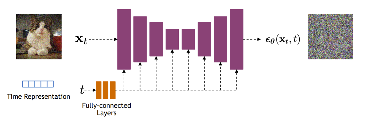
Architecture

Usually, we implement a diffusion model as a U-net that has a noise conditioning applied to every layer. The network predicts the noise $\epsilon_\theta$, or rather, the normalied noise. There are some technialities that i’m skipping here, but essentially this is a supervised learning problem

Diffusion Models as Hierarchical VAE

Iterative Noising (encoder)

So in our above derivation, we used samples with different noises added. We can represent this as a stochastic process where you start with noiseless image and you add noise iteratively through a conditional distribution

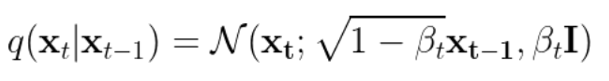
Therefore, you can sort of see this process as encoding some $x_0$ as noise. Every timestep, the encoder doesn’t have a parameter, but it still creates a distribution $q(x_t | x_{t-1})$.

As a sidenote, you can express $q(x_t | x_0)$ in closed form because of the gaussian formulation.

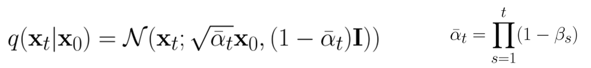
In total, you get a distribution over latent variables

Iterative denoising

In every denoising step, you want to compute $p(x_{t-1} | x_t)$. In diffusion, we use Langevin dynamics and a score estimation to sample from this distribuiton. We can reframe this as a heirarchical VAE, in which we have a chain of latent variables ($x_1, …, x_n$) that influence the main variable $x_0$.

In total, you get a decoder that takes these Latents and computes

Now this is tricky because you might think that we are re-modeling the latents. This is sort of true but note that we are taking the “encoded” latents and decoding every step, i.e. we are doing a chain of decoding. It may be more informative to think of it as two sets of variables: $x_0 → x_n$ as the encoding process, and then $x_n' → x_0'$ as the decoding process.

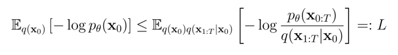
The ELBO

The ultimate goal is to still maximize $p_\theta(x_0)$, but this requires us to marginalize over $x_0,.., x_n$.

Concretely, we can compute $p(x_{0:n})$ easily using chain rule. We can also compute $q(x_{1:n} | x_0)$ easily using the noising equations. Therefore, the ELBO should come easily.

Relationship to score models

Let’s assume that we parameterize the denoiser $p_\theta(x_{t-1} | x_t)$ as a gaussian.

where the $\epsilon_\theta$ is a noise predictor.

The constants are derived from the noising process, which we don’t have to worry too much about (it’s a technicality). Now, if we construct the ELBO, we get

Hey!! This looks familiar! It’s just denoising score matching again!

Diffusion Models as ODE, PDE

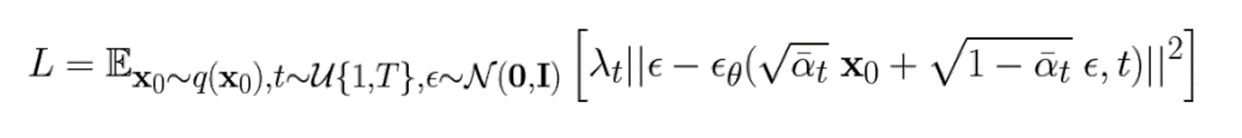
Diffusion as Continuous Process

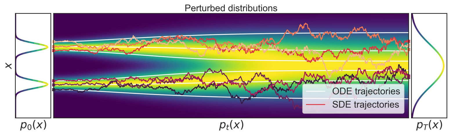
In this section, we will re-cast diffusion models as ODE’s, which gives us infinite noise schedules. So previously, we had imagined transforming the distribution as a stochastic process (Markov Chain, MCMC)

However, if you squint carefully, you can imagine a continuous process that maps the data to noise.

Diffusion as ODE

This discovery touches on a key insight: MCMC and stochastic processes are just a Monte Carlo solution to a stochastic differential equation! An SDE is expressed as the formula

where $t$ is the main variable, and $w$ is a noise component. All stochastic processes can be described this way!

In the diffusion model c ase, we have a forward SDE expressed as $dx_t = \sigma(t) dw_t$, and this $\sigma(t)$ is a continuous function now. This SDE is very simple: it’s just adding noise at every step.

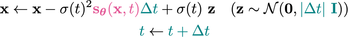
On the way back, we have a reverse SDE expressed as

Now, we don’t have to understand completely where this comes from, but do you see how we move in the direction of the score with some additional component of noise?

Training continuous diffusion model

Instead of conditioning the model on $\sigma$, you can condition the score model on $t$, which yields the following objective

It’s pretty simple; you just sample from a continuous distribution now, which is derivable through standard equation solvers.

In reverse time, you can compute the derivative form, which allows you to apply SDE solvers. One common solver is Euler-Maruyama, which is like the Euler method but for ODEs.

Notice how this is similar to the MCMC formulation. The key difference is that we move forward in $t$ rather than staying at one noise level.

Predictor-Corrector Method

When you do score-based MCMC, you’re keeping the $t$ but refining the distribution at $t$. When you apply an SDE solver, you’re moving forward in $t$.

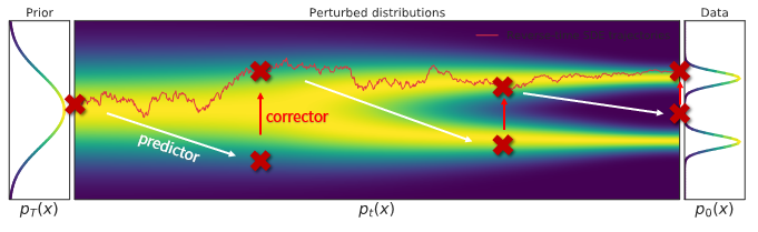
The process of moving forward (predictor) often makes mistakes, but the MCMC can correct for such mistakes. Therefore, a common algorithm involves running SDE and MCMC in an alternating fashion.

Converting SDE into ODE

It turns out that you can create an ODE (deterministic) mapping that creates the same marginals as the SDE. In other words, we can express this whole thing as a really complicated normalizing flow model!

Specifically, you can find this relationship

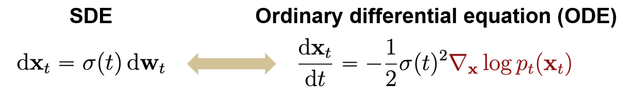
And you can invert this by computing

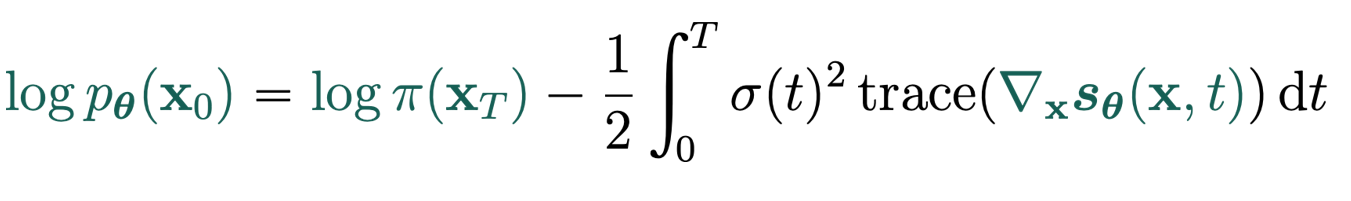
where the integral is computed by an ODE solver. So this is an continuous time normalizing flow model!

Distillation

The problem with a lot of diffusion models is that every step is very expensive. Therefore, we can train a good teacher that uses a lot of timesteps, and then you train a student model to mimic the denoising of multiple teacher steps at once. This helps with reducing the number of test-time denoisings.

Guided Diffusion

Latent Diffusion Model

Instead of generating an image, what if we generate a latent space? We can create supervision through a pretrained VAE.

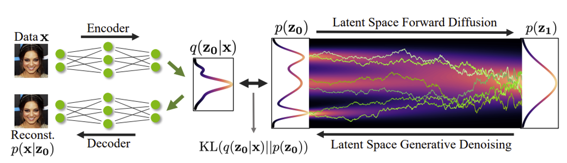
During test-time, this allows you to generate samples very quickly because you are in latent space. It can also be applied to discrete data.

Classifier Guidance

If you have some forward model $p(y|x)$ and some $p(x)$, you can create a diffusion model $p(x | y)$. This is because you can apply bayes rule for score funtions

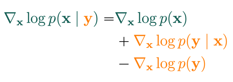
and the last term is zero. If you have $p(y|x)$ as a model (usually, $y$ is a class label), then you can easily compute the score of $p(x | y)$ and therefore train / sample from it.