The big idea

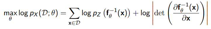
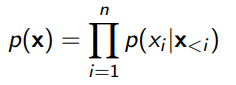
For VAE’s, we couldn’t compute $p(x)$ directly, which mean that we needed the ELBO objective to optimize it. Could we find some $p(x)$ that is complicated yet easy to compute?

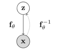
The key idea here is to find some invertible function $f(z) = x$ such that $p(x) = p(f(z))$. This is easy to compute and optimize over.

Background theory: transformation of distribution

When you transform a distribution, you need to scale it like this:

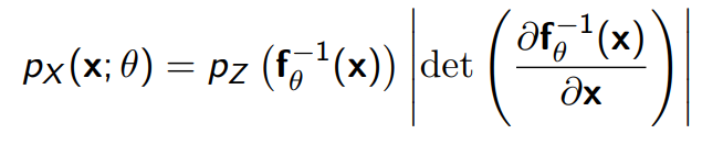
You can derive this through the CDF, but more intuitively:

• the determinant is how much the function x→z stretches.

• You want to divide the $p_z$ by how much the function z→x stretches

• The determinant of the function x→z is the same as the inverse of the determinant of the function z→x

The construction of normalizing flow

Functional Composition

If you had a bunch of invertible functions $f^i$, you can compose them into a more complicated but still invertible function

And using change of variables and a property of determinants/jacobians, we get

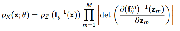
Concretely, this $z_m$ would be some data vector the same size as the final output. If this were an image, you would flatten it, or you might use a special convolutional function (more on this later).

Learning and using the model

• Learn through maximum likelihood by mapping the $x$ to the $z$ distribution and taking the likelihood. This allows for an exact likelihood evaluation

• Sample by taking $z\sim p_z$ and then computing $x = f_\theta(z)$.

• Get latent representations by computing inverse function $z = f_\theta^{-1}(x)$.

Desiderata

• we need a simple prior that can be sampled and evaluated on

• Easily invertible transformations

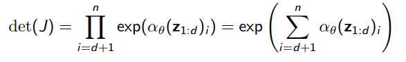
• Easily computable jacobian matrices (this is a really important one: normally a determinant needs $O(n^3)$ complexity, where $n$ is the data dimension. This could be really nasty.
  • Triangular matrix has a very simple determinant formulation

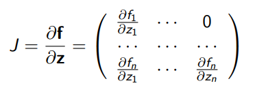
• A triangular jacobian means that $f_k$ depends on $z_1, …, z_k$, which is reminscient of an autoregressive model. More on this observation later.

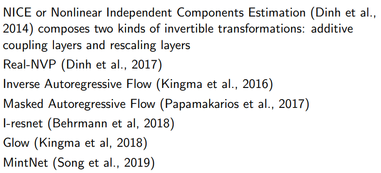
Implementations of Normalizing Flows

NICE (additive coupling layers)

The idea: partition $z$ into two parts: $z_{1:d}$ and $z_{d+1:n}$. Then, in the forward function…

• $x_{1:d} = z_{1:d}$

• $x_{d+1:n} = z_{d+1:n} + m_\theta(z_{1:d})$, where $m_\theta$ is any arbitrary function

As you can see, this follows the triangular formulation, and it is trivial to invert if you have access to $m_\theta$ and $x$: first, you get $z_{1:d}$ for free, which will easily allow you to compute $z_{d+1:n}$ from the $x_{d+1:n}$ and $m_\theta$.

The jacobian is very convenient: the diagonal terms are all ones, so the volume is preserved.

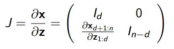
This also means that we don’t actually have to compute the determinant: $det(J) = 1$.

We assemble the NICE model by doing arbitrary partitions (so we have good mixing). The final layer applies a rescaling transformation by multiplying by some constant.

Real-NVP

Real-NVP is only a small step up from NICE, but we get much better results.

• $x_{1:d} = z_{1:d}$

• $x_{d+1:n} = z_{d+1:n} \odot\exp(\alpha_\theta(z_{1:d}))+ \mu_\theta(z_{1:d})$, where we have two neural networks.

As before, we can derive the inverse by computing $z_{1:d}$ for free, and using it to reverse the scale/stretch operation and get $z_{d+1:n}$.

The jacobian is slightly more involved, but it’s still very simple

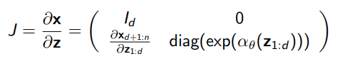
which means that the determinant is just

Unlike NICE, this is NOT a volume-preserving transformation. But it produces much better images.

Autoregression as Flow

So in creating our triangular Jacobian matrix, we had an interesting observation: this formulation looks really close to an autoregressive model! Let’s establish this fact a bit more

Masked Autoregressive Flow (MAF)

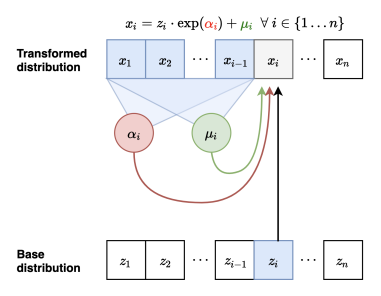
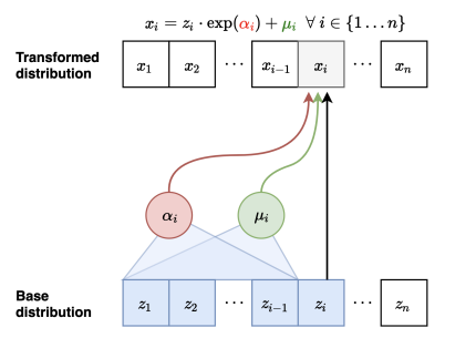
Suppose you had

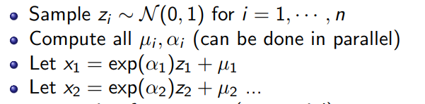
where each $p(x|x_{<i})\sim N(\mu(x_{<i}), \sigma(x_{<i}))$. To sample, you can use a reparameterizaiton trick. First, you sample a vector of $z$ (gaussian). Then, you would autogressively compute each $\mu, \sigma$, and scale the $z$ to form $x$.

• Concrete steps

  

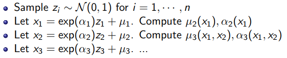
The flow interpretation is this: You take samples from $z$ and you map to $x$ using these invertible transformations parameterized by $\mu, \alpha$. This is really similar to real-NVP and NICE.

The inverse mapping, however, is really fast. If you had all $x$, you can compute $\mu, \alpha$ in parallel. This allows you to derive the $z$ quickly. Hmm..this is interesting. We have…

1. Slow forward mapping from $z→x$ because of autoregressive

2. Fast inverse mapping from $z→x$ because of parallelizable operations

Concretely, this means that this is fast to compute likelihoods and slow to sample from. It’s actually inverted from the best case scenario: it’s fine if it trains slower, but we want fast sampling. This brings us to an inversion of the structure

Inverse Autoregressive Flow (IAF)

The key idea is this: in forward flow, we created an autoregressive relationship in $x$, which created the problem with sampling speed. What if we made an autoregressive relationship in $z$? By using the sliding window, we still get the autoregressive dependence structure in $x$. However, because we know all the $z$’s ahead of time, we can compute the weights in parallel

The sampling process:

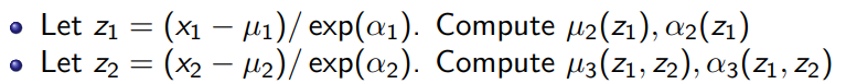
Now, the inverse mapping is slower. There is no free lunch. To derive $z$, you need to invert the $x$, and then use the solution to compute the autogressive parameters to get you the next $z$. The inverse mapping process:

This is fast to sample from and slow to train. Side note: because the generations come from $z$, it’s easy to compute the likelihood of the model’s own generations by caching the $z$.

Getting the best of both worlds

We know that the forward inference model is fast to train but slow to infer. Can we use this forward inference model as a teacher to teach an inverse inference student model that is slower to learn but fast to infer?

• this is possible because the student can judge the likelihoods of its own generations easily through a cached $z$.

You distill the teacher by matching the KL divergence of the student and the teacher. You sample from the student because you can easily compute likelihoods through caching. Computing likelihoods through the teacher is not a big deal because that’s the fast part.

Diffusion models as flow, flow as score functions

You can interpret (hand-wavy) diffusion models as a flow model, which also means that the flow models is an approximation of a score function.

Other Structures

Mintnet (Song et al. 2019)

• invertible neural networks using masked convolutions (allows us to apply this framework to images)

Gaussianization flows (Meng et al. 2020)

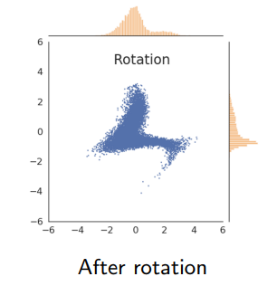
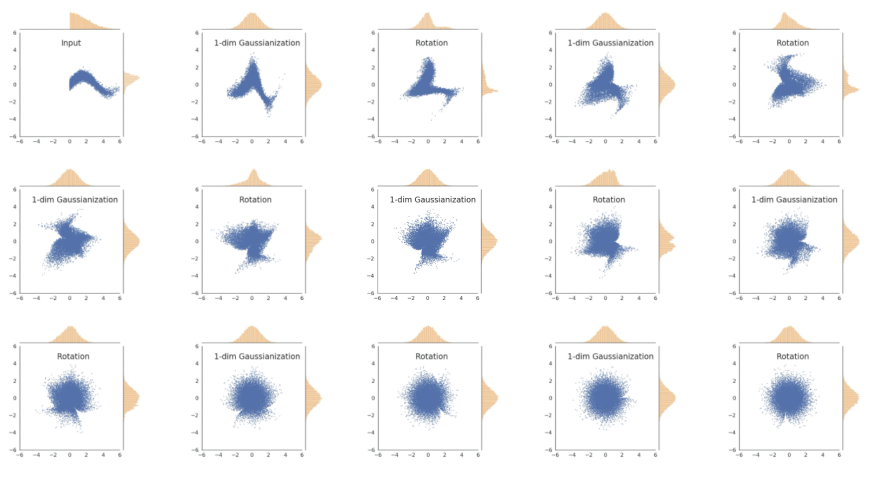
The idea is to map the data such that the marginals are gaussian. Then, we rotate the distribution to make it non-gaussian again.

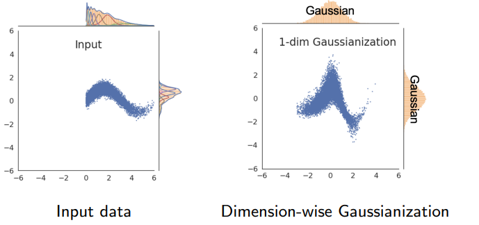
We do this by composing $\Phi^{-1}\circ F_{data}$, where $\Phi^{-1}$ is the inverse gaussian CDF and $F_{data}$ is the data CDF. This is valid because composing any random variable with its CDF makes it into a uniform distribution. Composing a gaussian function with its CDF makes it uniform, so composing the uniform with the inverse CDF makes it gaussian.

If we do this multiple times, you can transform any data distribution into a gaussian because the true gaussian is rotationally invariant! It is a fixed point of this functional process.

• Visualization

  

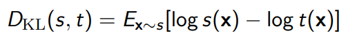
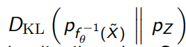
And this formulates your $f_\theta^{-1}$, and there’s a nice trick: you can use the KL directly, because

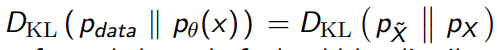
And applying an invertible function doesn’t change the KL divergence.

This is easy to compute because there is a closed form for a KL between two gaussians.

Literature and other works