Advice

• The form $E[\log p/q]$ isn’t necessarily KL divergence, although it takes a similar form

• For more complicated proofs, it helps to work backwards from the more complicated answer

• write out the expectation as a summation

Math review, proof tips

Jensen’s inequality: $E[\log(f(x))]\leq \log E[f(x)]$, opposite way around for convex functions. Useful because usually putting the log inside can create a simpler expression. This is your friend.

Mapping between distributions: $g(Y) = f(h^{-1}(Y))|\nabla_Y h^{-1}(y)|$, where $f$ is potentially a simpler function, $h$ is a mapping from simple to complicated, and $Y$ is the complicated distribution

Fenchel conjugate: the convex conjugate of a function: $f^*(t) = \sup_u (ut - f(u))$.

F-divergence: Anything of the form $D_f(p, q) = E_q[f(p/q)]$. The $f$ is lower-semicontinuous, i.e. points below are continuous. F-divergences are alwayas greater than zero.

KL divergence: $E_p[\log p/q]$

Bayes rule (duh): $p(x | y) = \frac{p(y|x)p(x)}{\sum p(y|x)p(x)}$

Subtract a KL trick: you know that KL is never negative, so if you can add / subtract, you can provide a bound.

Showing minimization, etc: see if you can rearrange into KL divergence or some other f-divergence. To do this, start with the difference (i.e. the optimal should be 0).

Distribution tricks

• marginalize → summation → potentially expectation

• Expand: $p(x) = p(x, y)/p(y|x)$. See if this gets you anywhere

• Marginalize: $p(x) = \sum_y p(x,y)$.

Expectation

• You can add an expectation out of nothing at all $f(x) = E_{p(y)}[f(x)]$. Look for these to turn functions into expectations

• Can write marginalization process as expectation: $\sum_z p(x, z) = \sum_z p(z)p(x | z) = E_{z\sim p(z)} p(x |z)$

• Expectation is linear, like gradient and integral

• log-probabilities allow you to factor like sums

• Expectation out of summation if there’s a distribution. You can also use a surrogate distribution: $\sum p(x, y) = \sum q(y) p(x,y)/q(y) = E_q[p(x,y)/q(y)]$.

• Tower property: $E_{p(x,y)}[f(x, y)] = E_{x\sim p(x)} E_{y\sim p(y|x)}[f(x,y)]$. More formally, it’s actually $E_{p(x,y)}[f(x, y)] = E_{x\sim p(x)}[ E_{y\sim p(y|x)}[f(x,y) | x]]$, but in most cases this is implied.

Some Basics

Jensen’s inequality

• $E[\log(f(x))]\leq \log E[f(x)]$ (when in doubt, remember that expectation is the secant line)

Lower bound computation

• use Jensen’s inequality or subtracting a positive value (for example, KL)

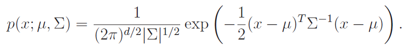
Gaussian formula

Expectation properties

• $E_{p(x, y)}[f(x)] = E_{p(x)}f(x)$

Divergences

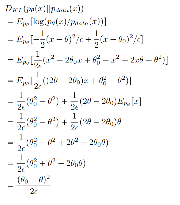
The KL divergence of two same-variance gaussians is simply the scaled square distance of the means

• Proof (just expanding the definition)

  

Estimators

An unbiased estimator of some parameter means that $E[\hat{A}] = A$ (and some convergence stuff surround this assumpation). Just because $\hat{A}$ is an unbiased estimator doesn’t mean that $f(\hat{A})$ will be an unbiased estimator of $f(A)$. It’s true for linear functions but not generally true for all functions.

Mapping between distributions / functions

This is a classic problem and it’s very tricky to understand. Here’s the setup: you have some known $f(x)$, some invertible mapping function $h(x) : X → Y$, and you want to find $g(y)$ as a function of $f(x)$.

Non-distribution setup

Without the question of distribution, this is actually really simple.

You take your $y$ and you map it into the domain that works for $f$. No biggie.

Distribution-based setup

Why doesn’t this work if $f$ is a density function? It has to do with density. Imagine the $x, y$ were rubber bands. if you have to stretch or shrink the rubber band in your mapping of $h$, then you run into the problem of having the same density with different scales, leading to a change in the integral.

More formally, if $dx \neq dy$, we’ve got a problem that we can solve with standard change of variable techniques. In calculus, we implemented these techniques when we mapped between two domains (u-substitution) but we wanted to keep the integral equivalent.

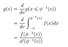
1. Start with $f(x)dx$

2. Find $h^{-1}(y)$

3. Compute $g(y) = f(h^{-1}(y))dh^{-1}(y)$ in terms of $y$, getting you the final answer

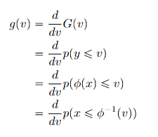
From this, we can derive a general rule (using the derivative of the inverse function general form):

• Proof (from first principles)

  

  

Generalization to vector-distributions

For vector distributions, we are dealing with a multi-variable transformation. This transformation, like the one-dimensional case, must be invertible. For a matrix, it must be full-rank.

Here, instead of worrying about $dx$ vs $dy$, we are worried about mapping $dv$ onto $dv’$, where $v$ is some unit element. As we’ve learned in multivariate calculus, the convenient notion is the Jacobian determinant, i.e.

Note how the forms are super similar; we just replace the derivative with the determinant of the jacobian. Recall that the jacobian describes how the unit-area stretches or shrinks with the transformation, so this is intuitive. So you’re almost “paying tax” by “unshrinking” from $y$ to $x$ before you apply the function.

Intuition

Let’s jump directly to the higher dimension.

1. $|\nabla_Y h^{-1}(y)|$ we know represents how much the space stretches as we apply the transformation from $Y→X$.

2. $f(h^{-1}(Y))$ is the density in X-space. If the Y→X increases, everything is naturally divided by $|\nabla_Y h^{-1}(y)|$ as we go into X-land. Therefore, to reverse this process, we multiply the value by$|\nabla_Y h^{-1}(y)|$

3. If Y→X decreases, the same logic applies, just with a $|\nabla_Y h^{-1}(y)|$ that is less than 1

You can think of a transformation as naturally dividing by the “stretch” factor $|\nabla_Y h^{-1}(y)|$, and you need to compensate as you map it back.

Worked example

If we have $p_X(x)$ known and we have a good function $f: X\rightarrow Y$, then we can compute $p_Y(Y) = P_X(f^{-1}(Y)) | f^{-1}’(Y)|$. Often, we get $f^{-1}$ at the start, which is fine. So, you just scale your values by $|f^{-1’}(Y)|$. If the operation is linear, this is a constant

• rule of thumb: if $X$ is a tighter domain, expect $p(Y)$ to be smaller. If $X$ is a looser domain, expect $P(Y)$ to be larger.

Convexity

Fenchel Conjugate

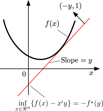
Any function has a convex conjugate known as the Fenchel conjugate

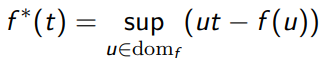
This is a generalization of Lagrangian duality, but intuitively, this is a convex hull to the function.

This $f^*$ is convex and lower semi-continuous. We can take more Fenchel conjugates, i.e. you can take the second Fenchel Conjugate

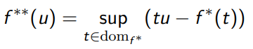
Properties of Fenchel Conjugate

We have $f^{**} \leq f$. If $f$ is convex and lower semi-continuous, $f^{**} = f$.

• Proof (definition)

  We know that $f^*(t) \geq ut - f(u)$, which means that $f(u)\geq ut - f^*(t)$. Therefore, $f(u) \geq \sup(ut - f^*(t)) = f^{**}(u)$.

F-divergences

Given two densities, we define a general f-divergence as

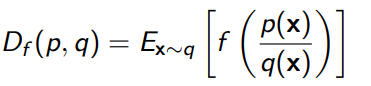
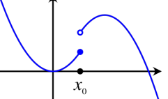
where $f$ is any convex, lower-semicontinuous function with $f(1) = 0$. Lower-semicontinuous basically means that around $x_0$, every point that is below must be continuous. Every point above is fine. This looks like the following diagram:

Properties of F-divergences

Always greater than zero

• Proof (convexity, Jensens)

  

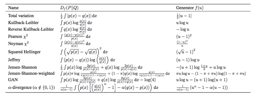
Examples of F-divergences

There are so many types of F-divergences, with a common type being KL divergence, where $f = u\log u$ (careful! It’s not $\log$ because it’s $p \log p/q$, not $q \log p/q$. ) Total Variation is also a common one, where the $f = |u-1|$