Moving from VAE, Flow

In MLE, variational autoencoders, and normalizing flow models, ultimately the objectives are based on minimizing KL divergence

This is a distance metric that decomposes into the log-likelihood. In MLE, we could compute it directly. In VAE, we used a special approximator. In Normalizing flow, we computed it through an invertible function.

Problems with maximum likelihood

In our previous approaches, we had some issues with computing likelihoods using the KL divergence. Furthermore, there are problems associated with maximum likleihood (i.e. KL divergence matrix).

If you have high likelihood, you can actually have a really bad model. By the log-construction, a sample that is noise 99% of the time and perfect 1% of the time will yield the highest score minus a (potentially) small constant.

Conversely, if you have good quality outputs, you can have low likelihood on the test set. A canonical example is an overfit model that memorizes the training set.

These counterexamples are yet another reason why we may want to shift away from the MLE objective; it seems to be a weaker objective than we want.

A learned metric (Discriminator)

What if we could replace the KL metric (which is rather dumb) with a learned metric? This is the idea of training a discriminator to tell the difference between $p_\theta$ and $p_{data}$.

We optimize this using a binary cross entropy objective, which looks like

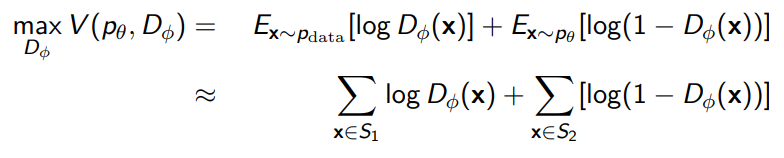
Now, this is tricky: an optimal discriminator satisfies

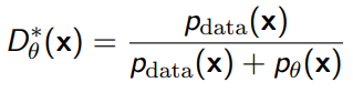
• Proof (expansion of expectation)

  

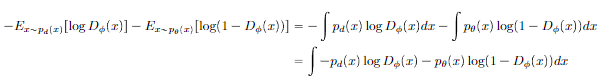
  If you take the inside of the integral to be $f(D_\phi(x))$, you’ll find that it only has one minimizer, and by calculus, you can derive that the minimizer is precisely $p_d / (p_d + p_\theta)$.

An optimal discriminator does not achieve perfect accuracy, because if there is a nonzero density in both distributions for some point $x$, it is ambiguous where the point came from.

Ultimately, this is a two-sample test objective to see if distributions are different.

A learned generator

You can learn a deterministic (potentially non-invertible) mapping $G_\theta$ between a low-dimensional $z$ and high dimensional data $x$. This is just a feed-forward network that takes a sample from the prior and outputs the generated output.

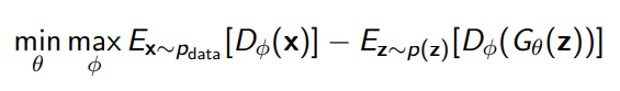
The Min-Max Game

We can frame the GAN training as a min-max game, where we do

Theoretical Interpretation

If we reach the true $D^*$ after each inner loop, then you can see that the objective $\min_G$ becomes the same as

• Proof (simple algebra) ‘

  Just substitute in $D^*$ and do some easy algebra to get the final result

  

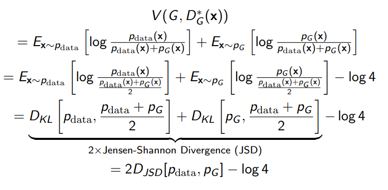
where JSD is a symmetric form of distribution divergence that is symmetric and has the properties of KL divergence

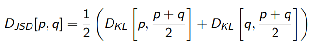
Namely, that $D_{JSD} = 0$ iff $p = q$, so we conclude that the optimal generator for the outer loop is $p_G = p_{data}$.

In reality

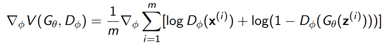
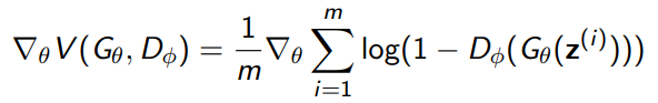
Even though the GAN looks like it can converge on this outer loop objective directly, bear in mind that every time we compute $\theta$, we have to recompute $D^*$.

In practice, however, it would be impractical (or downright impossible) to compute the inner loop to convergence, much less compute it for every $\theta$. Therefore, we do a sort of double optimization where we take the gradient WRT $D$, and then WRT $G$, and alternate. The gradients are easily computable:

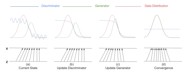
There’s a nice visualization of what the GAN does. It’s almost like a game of leapfrog

• Visualization

  

f-GAN

So far, we’ve trained with KL objective and JS objective. With JS objective, we found a way to avoid evaluating the likelihoods of the data, making it easier to train. Can we find a general method for all f-divergences?

tl;dr the big objective is to minimize an f-divergence without calculating the densities (and using samples instead).

Yes! With a Fenchel conjugate. Because $f$ is convex and lower-continuous, we have $f = f^{**}$.

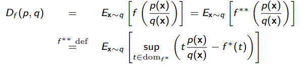
And we can express this supremum as a function $T^*$. This is unfortunate notation because the $*$ is also the Fenchel conjugate, but these are not related.

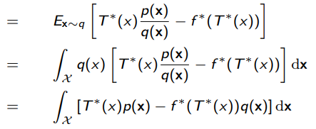
Now, this $T^*$ is also the function that reaches pointwise the highest for every $x$, so we can replace it with $\sup_T$, which is selecting a function from an infinite function class. We can narrow the function class, yielding a lower bound.

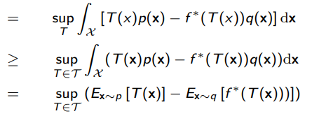
So we get a variational lower bound

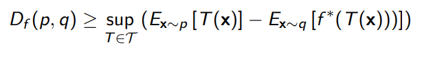
And this is really interesting! The lower bound is the summation of two expectations and $f^*$, which is some sort of function. Does this look familiar? It’s just a GAN objective hidden in plain sight!

To optimize, you need to maximize the inner objective ($\sup_T$) and then minimize the outer objective (which is the f-divergence)

Problems with f-divergences

If the $p, q$ don’t share the same support, we could run into issues. If $p(x) = 0$, we might get a really high (or infinite) value, depending on how things are defined. There may be sharp discontinuities that hinder training. Can we make a smoother objective?

Wasserstein GAN

The Wasserstein distance

We define the Wasserstein distance, or the “earth mover” distance as

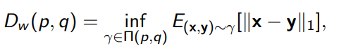
Intuitively, if you imagine the distribution as piles of dirt, this is the smaller amount of dirt you have to displace to turn $p$ into $q$. The $\Pi(p, q)$ is the set of joint distribution with marginals of $p, q$. The conditional model $\gamma(y|x)$ is the earth-moving model.

Of course, this is just intuition, and there’s a degree of formality that shows a similar thing. We can show that

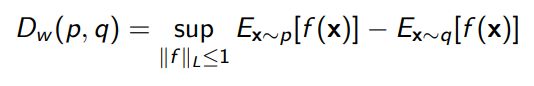
where $||f||_L$ is the lipshitz-number of $f$. Intuitively, we restrict the Wasserstein to classes of functions that don’t change very quickly.

Because we can write $D_w$ as this objective (known as the Kantorovich-Rubinstein duality), we can also optimize a Wasserstein GAN using this formula

where we enforce the lipshitz property of $D$ by clipping the weights or gradient penalty. Tl;dr if you clip the weights of a GAN or regularize the weights, you have made a rough approximation of a Wasserstein GAN.

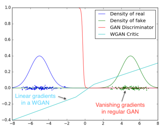
• Demonstration of smoothness

  A WGAN yields a much smoother transition boundary, which prevents vanishing gradients

  

Latent Representations in GANs

Unlike other models, the GAN does not have a mapping from $x → z$.

• solution 1: Feed $x$ into the discriminator and use one of the layers as the feature representation. The con is that the discriminator may not be looking for very rich features and you may not get something good

• solution 2: can we co-train an encoder?

BiGAN

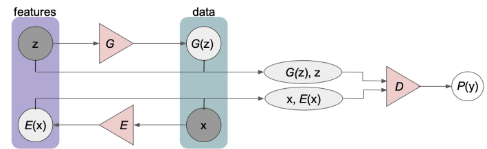
Previously, the discriminator is telling the difference between $G(z)$ and $x$. Now, we add an additional objective to tell the difference between $E(x)$ and $z$. This gets us a good encoder and decoder.

Domain transfer

We can use GANs to transfer between distributions, because we never restricted $z$ to be a simple distribution. We can have two very complex distributions, and the model translates between them.

We can start with paired examples and have the discriminator tell the difference between $y_i$ and $\hat{y}_i$.

You can also use unpaired examples, which requires a slightly more complicated structure (CycleGAN)

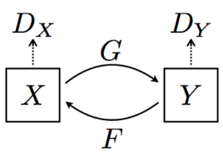
There are domain losses and cyclic consistency losses.

We may also preserve cyclic consistency using a cycle-consistent function to begin with, which is the idea behind AlignFlow.

Multiple domains

We can also make things more complicated by transferring between many domains. StarGAN accomplishes this through a central generator network and other objectives.

GAN problems

• Generator and discriminator losses can oscillate

• There is no robust stopping criteria (because there’s no global loss)

• There is no innate objective to prevent the generator to collapse its mode and always yield the same sample when queried. In fact, it happens pretty often on multimodal data.

https://github.com/soumith/ganhacks

https://github.com/hindupuravinash/the-gan-zoo