Density Metrics

Direct evaluation

One obvious way of evaluating density is through likelihoods on test set, i.e. $E_{p_D}[\log p_\theta(x)]$.

We can interpret this as how well the model compresses the data. Thge Shannon compression can create codewords of length $\log 1/p_\theta(x)$ for each point $x$, and so the expected length is just $-E_{p_D}[\log p_\theta(x)]$. We care about compression because the smaller the expected length, the better the model has identified overall patterns (and therefore reduced the need of expressing it in the compressed Shannon code.)

The perplexity used in language models is

which is closely related to density estimatino.

Estimation of density

In some models like VAE, GAN, and EBM, there is no direct likelihood function. You can approximate the likelihood by taking some samples, create an empirical distribution, and using this empirical distribution to find the likelihood.

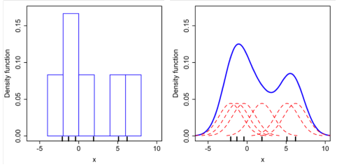
Naively, we can use a histogram binning method, where we create a bunch of samples and use the histogram (with some preset binning strategy) as a likelihood estimate. However, this a really coarse metric for high-dimensional data, where binning can be very hard (if not impossible, due to the sparseness of data).

Instead, we can do Kernel Density Estimation, which essentially takes the same samples, and then computes some form of distance metric that maps to likelihoods.

A common form is the Gaussian kernel, where $K(u) = \frac{1}{\sqrt{2\pi}} \exp(-\frac{1}{2}u^2)$. Unlike the Histogram, which needs an explicit binning strategy, the KDE only has the $\sigma$ bandwidth and creates a continuous density estimation

Kernels can take any shape and form, as long as they are normalized (proper density function) and symmetric. The bandwidth of the gaussian kernel controls how much smoothing will happen to the data, with large $\sigma$ being more smooth.

Unfortunately, both methods are unreliable in higher dimensions just due to the sparseness of data.

Importance Sampling

For conditional models, we can compute the likelihood by estimating the marginalization

This expression is unbiased for likelihoods for any choice of $q(z)$, but it is biased for log-likelihoods (if you just take the log of both sides).

Quality Evaluation

Human Evaluation

There is the HYPE metric, which asks humans to predict if an image is real or not. This is a good start, but human preferences may be hard to reproduce and potentially biased. Furthermore, there is nothing preventing the model from memorizing the training data.

Inception Scores

If you’ve trained the model on a labeled dataset and you have access to a classifier, you can compute the inception score. The inception score consists of two components

1. Sharpness: The more confident the prediction (classifier), the better. We do this by querying the entropy of the classifier $c(y|x)$ for every generated sample. The lower the entropy, the better.

2. Diversity: the more categories we generate, the better. We compute this by getting the marginal $c(y)$ of the predicted distribution. The higher the entropy of $c(y)$, the better. We compute this as follows:

The inception score is just the product of the sharpness and diversity scores.

Distance Metrics

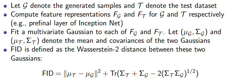
The Frechet Inception Distance (FID) by computing features (from a pretrained net) of the generated and test dataset. Then, we fit multivariate gaussians to these samples, and compute the Wasserstein-2 distance. The lower the distance, the better.

• Algorithm

  

The Maximum Mean Discrepancy (MMD) compares two distributions by looking at their moments (and cross-moments). We need some kernel as a measurement metric.

The Kernel Inception Distance (KID) computes the MMD in some representation space. It’s similar to FID, but it’s a bit slower but unbiased.

In general, there are a lot of different metrics we can apply to problems like these.

Latent Evaluations

Sometimes we generate latent representations of things. How do we evaluate the quality of such generations?

Clustering

We can make clusters of the representations using something like k-means, and we can see how well these clusters match with some known property (like the data class labels).

• Completeness score: are all points of one class in the same cluster?

• Homogenity score: are all the points in a cluster belonging to one class?

• V-measure: normalized mutual information, harmonic mean of completeness and homogenity scores

Reconstruction

We can look at how well the latent represents an element of the data distribution without losing information (and here you can use MSE, signal to noise, etc).

Disentanglement

Basically, does each axis of the latent variable correspond to a different feature in the output space? There are many qualitative metrics, but there are also quantitative metrics