What’s wrong with existing paradigms?

Because we model probability distributions, we restrict model architectures to outputting distributions. Usually this takes the form of parameterizing a gaussian, which is OK, but it’s tricky. We had to jump through a ton of hoops to get things like VAE’s working.

Energy-Based Models (EBMs) have flexible model architectures and have stable training properties. However, these are tricky because the output of the EBM doesn’t sum to 1, which makes it an improper distribution.

Master summary

1. EBM is a very straightforward thing to define

2. Sampling is hard from EBM, so is computing the likelihood

3. We can train through contrastive divergence, which requires model sampling

4. Computing gradient (score) is easy, so we can train using score matching

5. We can also use some tricks to train with noise contrastive estimation or adversarial optimization

Parameterizing Probability Distributions

If you have some function $g_\theta(x)$, you need to normalize it with a partition function $Z(\theta)$ to create $p_\theta(x) = g_\theta(x)/Z(\theta)$.

Composing distributions

The product of normalized functions is also a distribution, so you can do something like $p_\theta(x) p_{\theta’(x)}(y)$. The parameters can depend on previous generations; that doesn’t change the validity.

The convex mixtures of normalized functions is also a distribution.

The tl;dr here is that we can compose functions together, allowing for complicated expressions that are still probabilities. This can be helpful if you can find functions whose partition functions are analytically computable, like the Exponential family. These functions are simple but composable.

Exponential Families

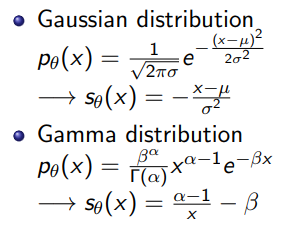
The exponential family are a family of functions whose partition functions can be analytically computed. These include Normal, Poisson, Exponential, Bernoulli, Beta, Gamma, Dirichlet, etc. These are nice, but they are not very expressive. Can we do better?

The Energy Based Model

We define the energy-based model as

This is helpful because the log-probability accesses the function directly, meaning that the gradients for the log probability are gradients of the function. Therefore the gradients will remain strong.

Pros and cons

Pros: this is very flexible— you can use any $f(x)$ you want

Cons: if you don’t have the $Z$, you can’t sample, evaluate, or even extract features.

The only thing you can do with $f_\theta$ is take the ratio of probabilities, because the ratio removes the partition function.

However, even this ratio may be very useful for classification, abnormality detection, and denoising.

We can also take the product of these unnormalized models to create the intersections of the energy fields, i.e. if you had $f_1*f_2 * f_3$, you’d be selecting for something that has all three properties.

Restricted Boltzmann Machines

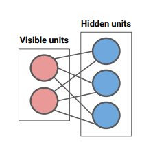
The RBM is a simple, older version of a generative model. There are visible and latent variables, both with binary values. We model the joint distribution as a second order function

Note how all the relationships are between the visible and the hidden; there are no relationships between the hidden units, or between the visible units.

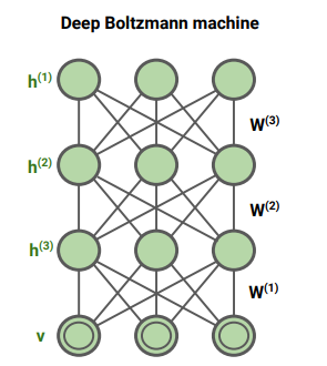
We can stack these on top of each other to create multiple layers of RBMs, which was a helpful pretraining objective for neural networks.

Training through Sampling

Our goal is to do maximum likelihood, i.e. $\exp(f_\theta(x_{train}))/Z(\theta)$. To do this ,we want to increase the numerator and decrease the denominator.

Notice that it isn’t sufficient to just maximize $f_\theta$, because it may pull up other things too, and that would make $Z(\theta)$ larger. We want to selectively emphasize the seen data point, which means that we need to push down the wrong points too.

Constrastive Divergence Algorithm

We start from first principles, which is essentially the KL divergence / log-likelihood objective:

Using log rules, we get

And using the definition of $Z$, we can get the following:

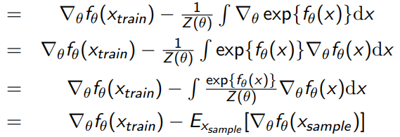
Note that the last step is because we recreated the model’s own distribution. We can estimate the expectation with Monte Carlo, which gets us the final objective of

So as long as we can sample from the model, we can improve it. We don’t have to compute the likelihood! And this is important because often, likelihood computation is worse than sampling.

Sampling

For sampling, we can avoid computing the partition function by using Markov Chain Monte Carlo (MCMC), which is a stochastic process that, when defined right, has a stationary distribution that is exactly the distribution of the energy function. This allows us to initialize the chain with a bunch of $x$, let it mix, and then pull out the $x$’s that have been changed into the proper distribution.

Normal MCMC

Concretely, these are the steps:

1. Initialize $x^0$

2. Let $x’ = x^t$ + noise.

3. If $f_\theta(x’)>f_\theta(x^t)$, let $x^{t+1} = x^t$ (stationary, i.e. you’ve gotten worse)

4. Else, let $x^{t+1} = x’$ with probability $\exp(f_\theta(x’) - f_\theta(x^t))$ (transition). If not, keep $x^{t+1} = x^t$.

5. Repeat steps 2 through 4 until we get stationary distribution

Note how 2, 3, 4 create a Markov Chain, with 3 and 4 representing two separate states that we transition to stochastically. This is how we sample, although it can take a long time to converge.

The theory states that we converge to $p(x)$ because satisfies the detailed balance condition, which basically states that $p_\theta(x)T_{x→x’} = p_\theta(x’) T_{x’→x}$, i.e. the distribution $p_\theta(x)$ is stable. There’s more on this in the 228 notes, so let’s leave it at this for now.

Langevin MCMC

Now, what if we can compute $\nabla_x \log p_\theta(x)$? This seems like a logical next step, given that MCMC was basically doing noisy gradient ascent. Well, if you have the score function, you can compute the following algorithm:

where $z$ is a noise scheduler. Note that energy-based models have a very easily computed score function:

So if we do this, we can essentially recover an objective that is similar to diffusion models.

Why is sampling bad?

Sampling suffers from curse of dimensionality—it takes a long time to converge for higher dimensions. Now, this is a problem because the sampling-based training algorithms will therefore require a lot of computational power to work. Can we do better?

Training through Score Matching

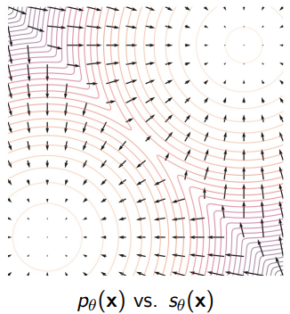
Score function

As we hinted before, it’s particularly easy to compute the gradient of the probability using an EBM because the partition function is agnostic to the value of $x$.

• Example of score functions

  

Score functions point to the place of highest density

Score Matching

So this is an interesting situation. We can compute the gradient of $p$ but not $p$ itself. It turns out, the Fisher divergence between two distributions is defined in terms of the score function

Now, we could formulate the objective of training EBMs as minimizing the Fisher divergence between $p_{data}$ and $s_\theta = \nabla \log p_\theta(x)$. If we define $p_\theta(x) \propto \exp f_\theta(x)$, then

Now, this poses a pretty large problem: how do we compute $\nabla_x \log p_{data}$? Well, we can try expanding out the squared norm and then integrating by parts. The integration by parts shifts the gradient away from $p_{data}$, which allows us to transform it into an expectation

• Good example with a univariate case

  We start by expanding out the objective

  

  And we take the $\nabla_x \log$ using the definition of the log

  

  And finally, we apply integration by parts

  

  (we assume that $p(x)→0$ at infinites.)

  Now, note how the blue term doesn’t depend on $\theta$ so we can essentaily push it into a constant. Therefore, we get this objective

  

  Note how this is computable through samples from the dataset and gradients of the EBF (which are directly computable).

If we do this derivation out in the multivariate case (which requires the multivariate variant of integration by parts), we get

which we compute easily through Monte Carlo estimation and gradient of EBF

This works very well, but unfortunately the trace of the hessian is pretty expensive for large models. Therefore, we may want a slightly different score matching objective.

Note how KL divergence objective got us contrastive divergence, and Fisher divergence got us score matching

Noise Contrastive Estimation

Here’s another way of optimizing an EBM: we assume that the correct distribution is different from noise, so you can contrast it from noise. How does this help us? Well, let’s try training a discriminator to tell the difference between data and noise

The optimal discriminator is

Ooh but this is interesting. So what if we parameterize the discriminator as the following?

This assumes access to the noise type, which is pretty reasonable (because you’re injecting it)

Now in this case, if we have an optimal discriminator, we are implicitly learning

so $p_{\theta^*} = p_{data}$. As another way of understanding this, we can rearrange to form

We can also interpret this formula as a “fix” or a “boost” to $p_n$, so if you started from a poor generation model, you can make it better with a well-tuned discriminator.

Training Approach

The problem is that $p_\theta$ has a partition function, which may not be tractable

What if we just trained $Z$ alongside? Well, we can rearrange the discrimnator as

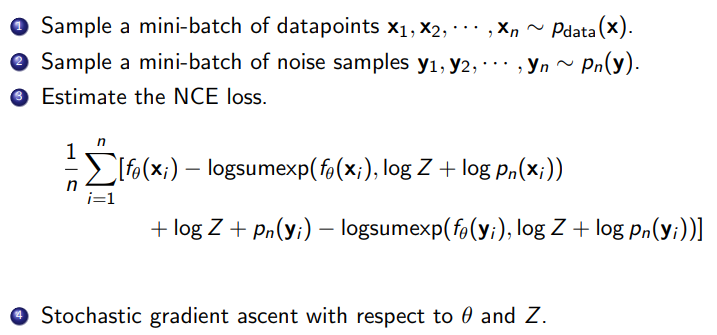
Now, if we plug this formula into the training objective, we get

Concretely, this is all computable, so we can just optimize through samples from data and noise

• Algorithm

  

Again, there is no need to sample from EBM

Comparing and contrasting NCE, GAN

Both NCE and GAN are training a classifier and are likelihood free (the GAN avoids computing the likelihoods)

However, NCE doesn’t need adversarial training, which means that it’s more stable. NCE also requires full access (likelihood) to the noise, while the GAN only requires samples (from either distribution).

Ultimately, NCE trains an EBM while a GAN trains a deterministic sampler. The big pro is that we also get an estimation of the partition function, which enables us to reconstruct the true distribution $p_\theta$.

Moving it back to contrastive (Flow contrastive estimation)

The observation is that we want $p_n$ to be as close to $p_{data}$ as possible to create a good discriminator. So, we can re-introduce the GAN objective! We can use a flow model to define $p_n$, which creates the following adversarial example

Adversarial Paradigm / Variational Paradigm

If we have an EBM, we can create a Variational estimation for $p_\theta$, which is easily optimizable

And the objective becomes

This $q_\phi$ needs to be a real distribution, but we can parameterize it (like a parameterized normal)

Good reference

https://arxiv.org/abs/2101.03288 How to Train Your Energy-Based Models