Caring about discreteness

There’s a lot of discreteness around us, and a lot of structures like graphs are also discrete. How do we model such structures?

Refresher: likelihoods on discretes

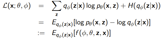
On continuous variables, we know how to get the likelihood $p(x)$ by just evaluating the model. Therefore, optimizing likelihood is akin to maximizing $\log p_\theta(x)$.

But what about discrete? Well, discrete models are just categorical distributions, so you’re more like looking at a whole list $p(x)$ and reading out the value at $x$. Maximization is akin to minimizing a distribution loss metric to a ground truth (like one-hot) key distribution. Actually, you’re doing the same thing when you’re doing MLE in the continuous space.

We can represent discrete distributions as a giant tabular distribution, but there may also exist other cool ways of parameterizing.

We can also think of discrete distribution samples as a $k$ dimensional one-hot vector. Contrast this with a k-dimensional sample from a continuous distribution, which has a lot more options. In both scenarios, each vector has an explicit density and that’s encoded in the distribution. This interpretation is a good unifying model for continuous and discrete distributions.

Derivatives Through Expectation

The problem with discrete latents

So previously, when we dealt with latent variable models, we often needed to compute something like this

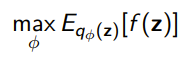
For example, in a VAE, we needed to compute an expectation over $q_\phi(z | x)$. For that, we used the reparameterization trick to compute the gradient. But what if $q_\phi$ can’t be reprarameterized as easily as a gaussian? Actually, one of the big problematic distributions are discrete distributions, which are generally hard to reparameterize.

Log Derivative Trick

There are two failure cases for the reparameterization trick: either $q_\phi$ can’t be reparameterized, or $f(z)$ isn’t differentiable. The latter case comes when $f(z)$ is some sort of reward function. However, in RL, there exists policy gradient methods that can solve a similar objective. These policy gradient methods use the log-derivative trick.

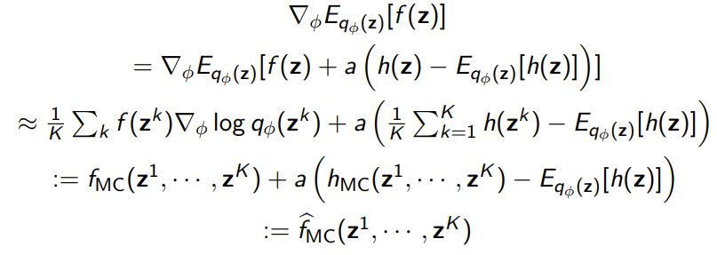
This trick takes advantage that $\frac{d}{dx}\log x = \frac{1}{x}$ and a multiply-by-one trick.

This helps us because we expressed a gradient of the expectation distribution as an expectation! Now, we can estimate it through a Monte Carlo sample!

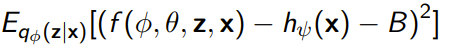
Control Variates

Because we rely on Monte Carlo method, the log derivative is often very high in variance. We know this to be a problem in reinforcement learning.

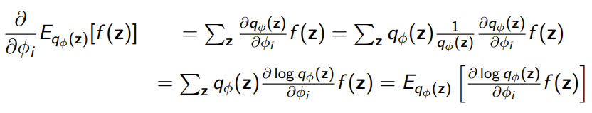
To resolve this, we often subtract some baseline from $f(z)$ (we do this in RL as well), and this is known as a control variate

• Proof that CV doesn’t make gradient estimation biased (calculus)

  

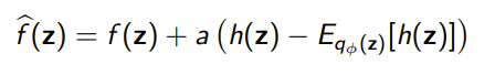
In practice, we use some control variate $h(z)$ that we use to define a new $\hat{f}$.

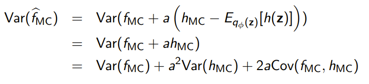
• Proof that this reduces variance (algebra, optimization)

  Which means that we can derive a new gradient estimate

  

  We can compare the variances of $\hat{f}$ gradients and $f$ gradients, which yields

  

  Which means that we can optimize for the $a$ to minimize the variance. Note that this $a$ is negative.

  

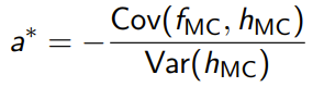
  And if you plug this back into the definition of $Var(\hat{f}_{MC})$, we get

  

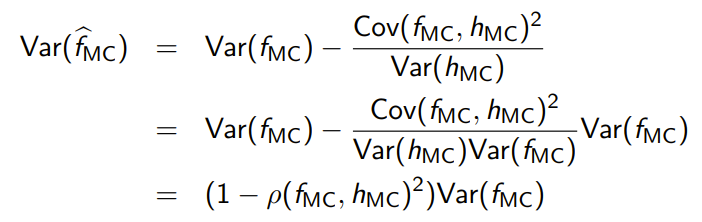
  Where $\rho$ is the correlation coefficient between $f$ and $h$. Note that this is between 1 and -1, Therefore, $1 - \rho^2$ will always be at most 1, and the more correlated we can get $f$ and $h$, the lower the variance.

Belief Networks

Belief networks are networks that use discrete latent variables, and the objective is the same as the ELBO

Because $q_\phi$ is discrete, we need to use the log-derivative trick with control variates to reduce variance.

Neural Variational Inference and Learning (NVIL)

This is an algorithm that uses the method above. For control variate, they used a constant as well as an input-dependent $h_\phi(x)$, yielding the objective

Continuous Relaxation

Another option for discrete latent variables is to relax it into a continuous and reprameterizable distribution.

Gumbel Distribution

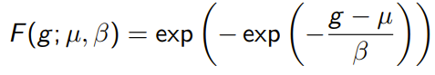
Given $n$ iid samples, what is the distribution of

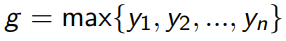
We call this a Gumbel distribution, and it models extreme events. It’s the exponent of an exponent, parameterized by location $\mu$ and scale $\beta$

Gumbel-Max Reparameterization Trick

Let $\pi$ be a categorical ditribution with probabilities $\{\pi_1, \pi_2, … \pi_k\}$. If you can sample from Gumbel(0, 1), then you can sample $g_1, …, g_k$ from Gumbel(0, 1). We assert that

is distributed like the categorical distribution $\pi_i/\sum_{j}\pi_j$. We can represent each sample as a one-hot vector.

This is the reparameterization trick because the computation of the arg-max is deterministic; the randomness comes from the Gumbel.

Gumbel-Softmax Reparameterization

Unfortunately, we can’t differentiate through an argmax, so instead we can soften the one-hot vector definition into a softmax

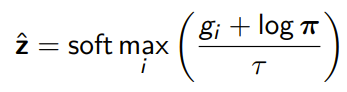
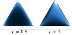
This temperature is a bias-variance tradeoff: the higher it is, the more correct it becomes. However, the variance actually goes up. The closer $\tau$ gets to $\infty$, the closer the samples become uniform.

Geometric Intuition

Why does this even work? Well, let’s imagine a distribution of $k$ categories. If we imagine that this is a k-dimensional space, categorical distributions place densities on the vertices.

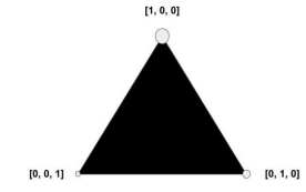
Gumbel-softmax will soften this by creating a distribution in this “simplex”

Using Gumbel-Softmax trick

Usually it’s enough to just use it in lieu of $q_\phi(z)$ and you control $\phi = \pi, \tau$, where $\pi$ is the categorical parameters and $\tau$ is the temperature. You usually anneal $\tau$ through time, starting with high $\tau$

If you really need explicitly categorical distribution when doing forward pass, you can use the straight-through gradient trick, which means that you use a hard categorical sample for forward pass and the GumbelSoftmax for gradients in backward pass.