Value Function Methods
| Tags | CS 234CS 285Reviewed 2024Value |
|---|
Moving from AC
Actor-critic we used a policy to act and a critic to change the policy. But can we do without the actor? This insight gives rise to a set of value-based methods.
Note that these will sound very familiar because we’ve talked about them in the Model-Free Control section. However, that section posed many different methods in a tabular environment. We will now turn to practical methods that work in real environments and deep networks. You will find that the ideas are very similar.
Policy Iteration
This is the first value function method we will talk about. The idea is very simple
- Fit using your preferred method (like TD). Typically this is done through a Monte Carlo estimate of
- Set as the delta function, where if
Practically-speaking, you only need to fit because and doesn’t depend on .
Connection to tabular, model-based methods
Recall that we had policy iteration in the tabular environment, where we alternated between learning a V function through bellman backups and deriving a policy from the Q function (which is in turn derived from the V function). So we are just doing the same thing, except that everything is approximate.
Value Iteration
Policy iteration can work, but we are still defining a policy explicitly. If we know that the policy is just the argmax, we can forgo this policy completely and arrive at the value iteration algorithm
- Fit . Approximate this expectation with a sample
- Fit
Note that the first step is evaluation, and the second step is improvement. The implicit policy of is better than the implicit policy behind .
Derivation of Q-learning
We can do step 1 and 2 in one singular optimization problem, where you define the target and then you fit to . We call this Q-learning.
Connection to tabular, model-based methods
As we saw in the tabular notes, value iteration is different because of its implicit policy representation. There are some subtle differences in behavior, as outlined in those notes. But overall, we are just re-establishing a method that we first talked about in tabular.
Dealing with the maximization
In discrete land, you can just ask the Q function for all the actions and pick the best. In continuous land, this might be a bit hard to do because you need to maximize. In this case, an actor critic algorithm might work better (although the tradeoff is that AC is generally on-policy)
Why fit V or Q?
The cautious reader may notice that our version of value iteration is different than the one in the tabular notes. Instead of fitting V, we fit Q and then maximize. It begs the question: why chose to fit Q or V?
It turns out, there’s one critical difference. Consider policy evaluation for V:

Note how the update requires you to have actions from , and this isn’t good if you’re using offline data of the form . But now consider policy evaluation for Q:

Do you see how it doesn’t matter what distribution is sampled from? It means that you can apply this algorithm to any interaction data and yield .
Therefore, if you want your algorithm to be off-policy, you would want to fit a Q function, not a V function.
The General Fitted Algorithms ⭐
For Monte Carlo, you use as the target

For SARSA, you use the TD target

and for Q-learning, you use the max-Q target (Known as fitted Q iteration).

Why Fitted convergence is hard
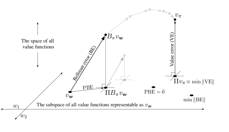
Essentially, when you are doing function approximation, you’re constrained to a subspace.
The bellman backup is a guaranteed contraction, but this backup may take you out of this subspace (see diagram).
Therefore, you have to project it back to the subspace with , and you can no longer say anything about this being a contraction on your subspace. You might actually be going further away.
Deep Q learning (DQN) 💻
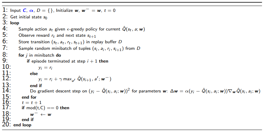
This is just Q learning with a slow-updating target function modification and the use of neural networks.
This isn’t stable out of the box though. We might get some divergence. There are two primary problems.
- Correlation between samples
- Non-stationary targets
In the next part, we’ll talk about how we can resolve such issues
Experience replay
The first problem is sample correlation. You ideally want IID samples from your policy, but your policy is rolling out in an environment linearly. So you’re going to get highly correlated samples, which can lead to sequential overfitting.
To solve this problem, just use a replay buffer! Q-learning is off-policy so we can learn from past experiences.
Generally, the more memory the better, although if your dynamics are changing, you might want a smaller memory.
Fixed Q targets
The second problem is that your target Q value changes with your updates because they share the same parameters (even if you didn’t propagate directly into it). This might lead to a dog-chasing-tail sort of problem.
To solve this, just freeze the target Q network and update once every updates to the actual Q network. However, this doesn’t necessarily solve another problem that arises with this framework, known as maximization bias. In the next part, we will talk about this.
Maximization Bias and How to Solve
What is maximization bias?
Well, intuitively, you’re trying to maximize the function, but this maximization yields some potentially harmful pitfalls. We’ll look at offline RL later where this is a big problem, but essentially when you maximizie the Q function, you may be accidentally selecting an accidentally high value.
More theoretically, you can consider Jensen’s inequality in this toy example, where we only have two actions and they both have zero expected reward. However, because of Jensen’s inequality, you have

So this estimation may be greater than , even though the true value is .
How does Maximization Bias affect learning?
Maximization bias can slow things down, and in functional approximation cases, can lead to suboptimality. However, in the tabular environment, GLIE is enough for convergence.
Double Q learning
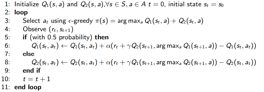
One idea: use one Q function to select the max action, and use another to estimate the value of this maximum action. Intuitively, we want to avoid using the max of estimates as the max of true values. By decoupling the selection and evaluation, we move in that right direction.

Double DQN
With DQN, there’s a lagging target and there’s the current network. With DQN, we maximize over this target network and then evaluate stuff on the target network. Can we use the same idea from Double Q learning here?

we can! Use the current network to select the best action, evaluate with target network, and update your current network.
With continuous actions
We can extend Q learning to continuous action spaces. The main problem is that the doesn’t work very well over continuous action spaces. We have three choices
Approximating the maximum with classic approaches
We can approximate the maximum over the continuous space as the maximum over a set of discretized values. The problem is that this is not very accurate.
We can use a cross-entropy method (see later lectures). It’s basically rounds of iterated sampling, and it’s pretty fast. These things work OK up to around 40D action spaces.
Fitting a simple Q function
We can also use a function class that is easy to optimize like a quadratic function

This is a neural network that gives a quadratic in terms of the action (NOT in the state, so it’s still pretty powerful). this method is NAF, or Normalized Advantage Functions.

This is efficient but it’s less expressive
Learn an approximate maximizer
We can train a second neural network that performs optimization. One example is DDPG, and essentially, you let be the negative loss and you try to optimize the second neural network to maximize this . This is sort a deterministic actor-critic algorithm.

We solve this using the chain rule:
Where is a jacobian.
Practical Considerations & Improvements
- use multi-step returns (although beware! this is no longer off-policy anymore!)
- try with toy examples
- Q learning performs very differently with different environments
- large replay buffer can help (roughly 1 million)
- it takes a lot of time; you might see signs of life much later
- bellman error gradients can be very large. However, if you have a very bad action, you don’t really care about how bad that is. However, the regression task will care a lot, which can lead to your gradient being swamped. Clip your gradients, or use a Huber loss

- double Q learning can really help
- schedule exploration and learning rate, as well as using things like Adam
- run multiple random seeds
BONUS: Heavy Theoretical Analysis of Fitted Q iteration (CS 285)
Recall that fitted Q iteration is defined as

We approximate this by doing it as an optimization problem

There are two sources of error: the is an approximate bellman operator (because it’s derived from approximate rewards and probabilities), and the minimization is approximate as well. This is called sampling error and approximation error respectively.

The is the average reward seen at this state-action tuple, and is the empirical transition distribution as derived from observation

What do we want to ask? Well, how close can we get our Q functions?

Sampling error
We want to understand this difference

If we sub the definitions, we get

By the triangle inequality, we get

Now, the first value is the estimation error of a continuous random variable, so we can use a concentration inequality

The second value we can factorize, and then we can bound

and this by definition is the total variation divergence of multiplied by the infinity norm of , which gets us

and using our derived bounds for categorical distributions, we get

So, we get that


Approximation error
Why don’t we assume that when we fit a function, our fit has an infinity error at most

(for now, we assume that we have an exact backup operator for a second)

^ this is just an add-subtract trick. We can group

and apply triangle inequality and definitions

The bellman backup is a contraction, which means that applying to two Q functions causes them to be closer by a factor of .

So, we’ve related the Q functions recursively:
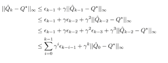
And at this point, we realize that the more iterations we take, the more we forget our initialization!

(we simplified the by replacing it with the maximum . So, the approximation error scales with the horizon too.
Putting it together
We have our sampling error and approximation error. How do we combine them?
Well, let’s do the same trick

The first term is approximation error and the second term is the sampling error. So, the total error is just these two errors added up

This tells us that
- error compounds with horizon
- Error compounds due to sampling
