Reset-Free RL

Tags	CS 224R

What do we care about?

In simulation, it can be pretty easy to establish an episodic setting, where you reset after every horizon limit. But in real life, this is hard to do (and often infeasible). We try to learn in one horizon, without resets.

Evaluations

In looking at reset-free or long-horizon RL, we care about two possible metrics

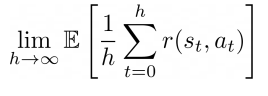
total reward (given that you live once, how can you maximize reward?). Known as continuing policy evaluation

goodness of policy (if you evaluate the policy learned in the environment, how well does it do?)

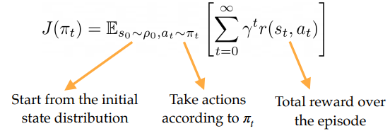
You can have a high total reward without learning something perfect. The reset-free paradigms typically target the second case, while the single-life paradigm typically target the first case.

Reset-Free

What’s the problem? Well, if you keep on running longer and longer horizons, the agent may just hover around the goal and never learn after that. We need a way to get us back to the beginning.

Forward Backward

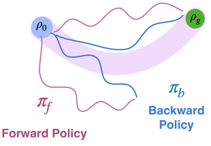
The forward-backward algorithm is very simple

Use forward policy to accomplish the task

Use backward policy to reset the environment

The backwards policy is easier to learn because at the very beginning, it’s easier to reset from a mess-up (most of the time).

Expert Distribution Matching (and curriculums), MEDAL

If we have the backwards policy, we can do more than just reset the environment. We can use it to reset to a place within the expert state distribution $p^*(s)$ , such that the forward policy might be closer to the goal. This helps the forward policy learn!

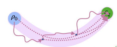
To do this, we optimize the objective $D(p^*(s) || p^\pi(s))$ where $\pi$ is the backward policy. We can accomplish this through a classifier.

The classifier predicts $C(s) = p(y = 1 | s)$ , where $y$ is the label. It’s either $1$ if it comes from the optimal policy, and $-1$ if it comes from the backward policy. Using bayes rule and the assumption that the dataset is balanced, then we have

C(s) = p(y =1|s) = \frac{p(s|y=1)}{p(s | y = 0) + p(s | y = 1)} = \frac{p^*(s)}{p^*(s) + p^\pi(s)}

And you can actually solve for the ratio

\frac{p^\pi(s)}{p^*(s)} = \frac{1 - C(s)}{C(s)}

Which means that

D_{KL}(p^\pi(s) || p^*(s)) = E_{p^\pi(s)}[\log \frac{p^{\pi}(s)}{p^*(s)}] = E_{p^\pi(s)}[\log \frac{1 - C(s)}{C(s)}]

and this is fully calculable as we have samples from $p^\pi$ and we have the classifier. In essence, to make this closer, we can just use that inner term as a reward augmentation.

Single-life RL

In this case, we care about the cumulative rewards. Therefore, we want to make sure that we don’t get stuck somewhere and don’t recover. To do this, we regularize the agent based on state familiarity, which gives it an incentive to do what it knows.

More concretely, we want to bias towards states seen in prior data. To do this, we train a classifier between prior data and online data. The reward during the single-life RL will be regularized by this classifier:

r = r(s) - \log(1 - C(s))

This is known as the QWALE algorithm.