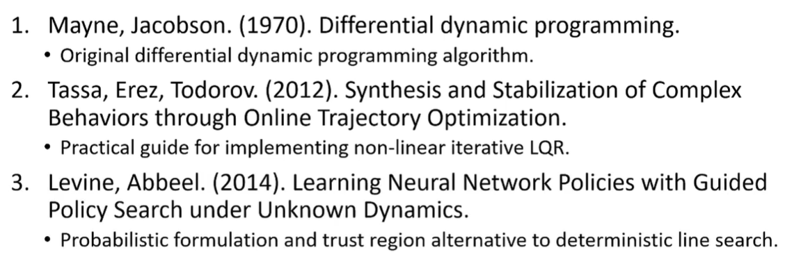
• Additional reading

  

From model-free RL

We assumed so far that the transition probabilities are unknown. But what if we knew them?

In some settings, you do know the dynamics. For example, the rules of a board game are known. Other systems can be easily modeled by hand, like driving a car. And in simulated environments, we have ready access to the dynamics.

But to use models, we need to learn about some optimization techniques used in optimal control.

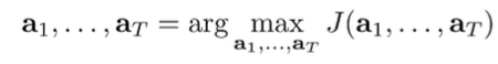
Open-Loop Planning (gradient free)

We see this whole thing as a black box, where you just need to find a bunch of actions that are good.

Of course, this is open loop, which has its disadvantages. You aren’t able to adjust for situations that aren’t seen in $s_1$, which means that your policy is not as adaptive.

Random Shooting

We can first try guessing and checking, known as random shooting. You do this for $n$ times, run it through the model, and you pick the best one.

Cross Entropy Method (CEM)

We can use a cross-entropy approach to essentially optimize across the actions iteratively.

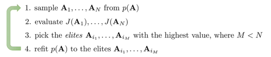
Unfortunately, this has a pretty harsh dimensionality limit (curse of dimensionality).

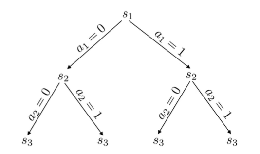
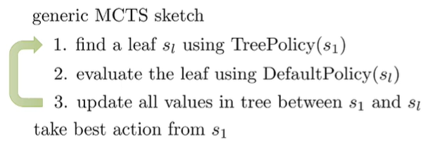
Monte Carlo Tree Search (MCTS)

You can basically make a search tree with different actions and different states (you know these states because you know the model)

This, of course, is not efficient as it blows up exponentially. To help, you can run some baseline policy to get a Monte Carlo return at that point. This allows you to estimate the value of that particular state without further expansion. If you land in a bad state, the baseline policy won’t do well, and if you land in a good state, the baseline policy might even do very well.

You start the search at $s_1$ and you expand it one step at a time. For example, you first step is to get to $s_2$ and then running the baseline policy. As you explore, you go deeper and deeper.

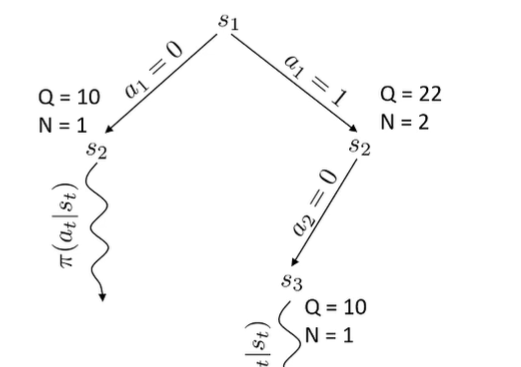
Exploring is not trivial, because you need to balance exploration and exploitation. To figure out which branch to explore, we can use a special score algorithm known as UCT. If $s_t$ is not fully expanded, then choose an action $a_t$ that has not been explored yet. If everything is expanded, pick the action that yields a state with the highest score, where the score is defined below:

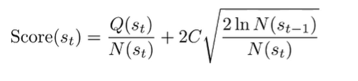
While doing this, keep track of $N$, which is the number of times you’ve visited this particular state. Also keep track of $Q$, which is the summation of total rewards. In other words, once you get a return (from the baseline policy), you add the return to all Q’s in that explored path.

You are basically exploring nodes of the tree that have high average returns (Q/N) or nodes that are more novel.

The final product is a tree with values for each action at each timestep. During eval time, you just pick greedily without the novelty boost.

Open-loop gradient methods

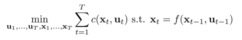
If we have a differentiable model of dynamics, we can try using a gradient-based method. As notation, we are trying to minimize cost (not maximize reward)

Shooting Methods

The optimization problem is just a constrained optimization problem

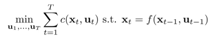
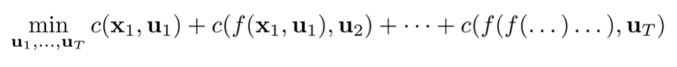
Because this is an equality constraint, we can substitute this constraint into the objective to get an unconstrained optimization problem

As long as $f$ and $c$ are differentiable, we could just differentiate through backpropagation and optimize! In practice, it helps to use a second order method. First-order methods often perform poorly due to the chaining of the functions.

Because you optimize over actions only, this is called a shooting method.Intuitively, this can be unstable because you’re not really setting waypoints for the trajectory; you’re just controlling the throttle, essentially. Therefore, even in a deterministic setup, it becomes harder and harder to plan for actions in the future (butterfly effect).

Colocation

For a colocation method, you minimize over both states and actions, or sometimes just states.

So because of the equality constraint, it isn’t a complete free-for-all. But the key insight here is that you get control over the waypoints, and the actions are just defined to get us to those waypoints. This gives us far more control and stability. Intuitively, even if you have a point $n$ steps away, you know that there is a waypoint $n-1$ steps away, and you can get from these points pretty easily by deriving the right actions. In essence, you’ve just shortened the action prediction horizon.

These methods are generally more complicated than shooting methods, and they are typically done in first order.

Linear Quadratic Regulator (LQR)

Let’s look, as a case study, a gradient control method that has a closed form shooting solution.

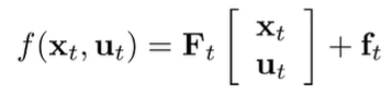
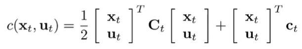
We start by using a linear dynamics model and a quadratic cost function.

Every timestep can have different $C_t, F_t$. We want to solve for $u$. naturally, because this is a recursive optimization formulation, we will try to develop a recursive algorithm to solve it.

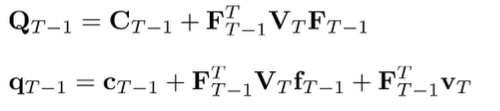
Deriving base case

Naturally, we try to solve for the last $u_T$. More specifically, we need to find a solution that is a function of the last state $x_T$, which will allow us to plug through the recursive case.

We consider the Q function at this timestep. The only part influenced by $u_T$ is the last one, so we have

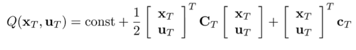
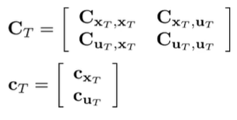
Because of the block matrix setup, we can split the reward like this:

And this becomes a standard matrix derivative problem. You get this gradient

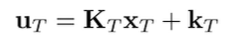
And you can set this to zero and get the following solution

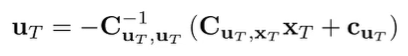
We will rewrite this value using $K_T, k_T$ for notational simplicity.

Now, if we assume we choose this $u_T$, we can get the value function of $x_T$ by plugging this $u_T$ back in.

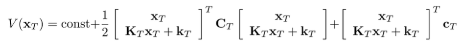
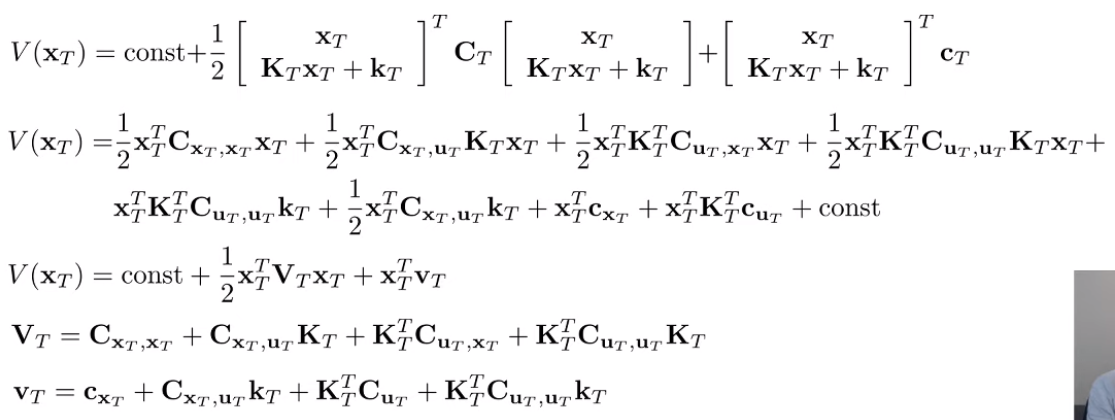
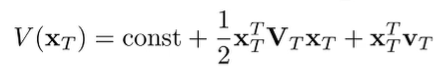
If you expand this out (it’s really ugly), you see that it’s still quadratic and you can consolidate things under a new matrix $V_T$ and vector $v_T$.

• Expansion

  

Recursive case

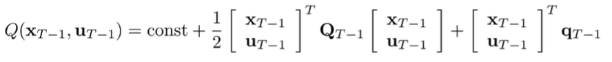
We want to derive a recursive algorithm. To motivate this, we will look at the previous timestep $T - 1$. We know that $u_{T - 1}$ influences $x_T$, so there should be an interesting dependency that allows us to plug in our base case.

We have a linear dynamics model, so we can use this to formulate our Q function

We plug in the definition of $f$ into the $V$ expression we derived above.

Now, if we put this back into the Q function definition, you’ll notice that you can combine the quadratic forms into one single quadratic form

where

And this allows you to optimize over $u_{T - 1}$ like we did above.

and this is the same form as our base case, so the solution is

This is significant because we showed how to optimize any $u_{t}$ using the solution to $u_{t+1}$. And this allows us to formulate the recursive algorithm.

The algorithm

We can express our solution as a recursive algorithm in optimization.

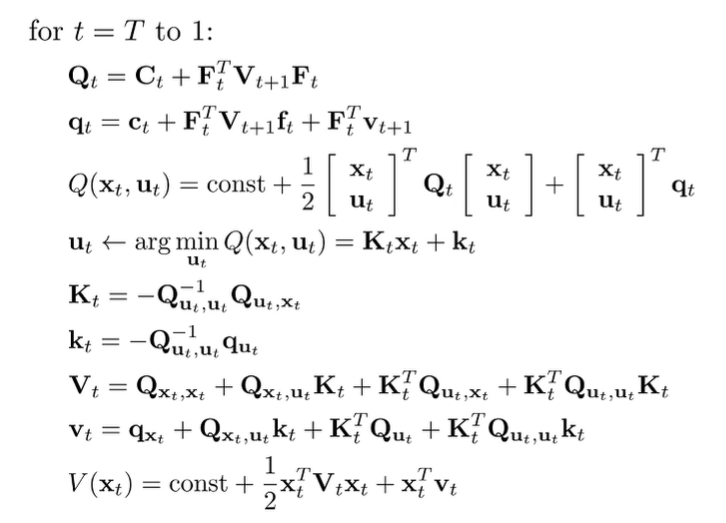
where the base case, $V_{T+1} = v_{T+1} = 0$.

Like all recursive algorithms, we build up a sequence of dependencies. Then, when we hit $x_1$, we know this particular value (it’s the initial state), which allows us to compute all of the future $u$’s through a cascade of our dependencies (forward recursion).

Extending to stochastic dynamics

Before, we had linear and deterministic dynamics. To add stochasticity, we can make a (potentially reasonable) assumption that the noise is gaussian centered around a linear mean.

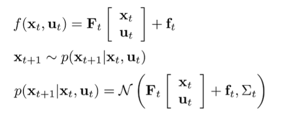
If this is the case, then the solution is actually the same. Intuitively, this is true because the gaussian is symmetric. However, because things are stochastic, you can’t produce an open loop solved series of actions. After you do backwards recursion, you need to run the policy in the environment. At every timestep, you use the relationships you derived in the backwards recursion to derive your next policy

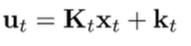
And every step, you pick your next policy.

Extending to nonlinear case (DDP / iterative LQR)

So interestingly, when we have non-linear systems, a lot of the stuff still holds. We just use Taylor approximations to create these locally-linear systems

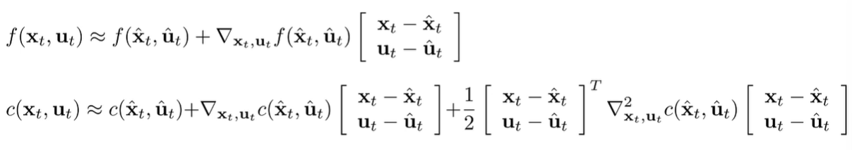
And therefore, we can express our systems as deviations where $\delta x = (x_t - \hat{x_t})$, etc

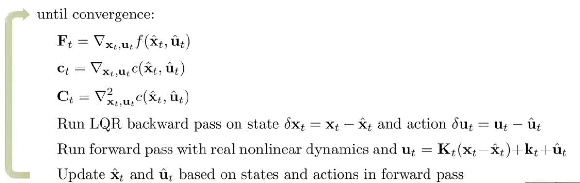
And if we can get closed form expression of the derivatives for any $x, u$, then we’re back in familiar LQR territory. The only difference is that we’re dealing with $\delta$’s, not absolutes. These $\delta$’s tell us which direction we want to perturb the $x, u$ to reach optimality under the current assumptions $x_t, u_t$. So we start with some initial guesses for all $x_{1:T}, u_{1:T}$. We compute the LQR at this guess, which gives us a forward policy.

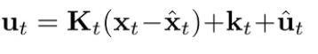
We run the forward pass with the real non-linear dynamics, which gets us a new set of $x_{1:T}, u_{1:T}$. This is our new guess, and we are ready to run LQR on it again.

We don’t just use the $\delta$’s to refine our initial guess because these are subject to local linearity, which may not be correct. Instead, we get “online” data by running the forward policy.

• General algorithm

  

Why does this work? Well, it’s actually similar to Newton’s method. In Newton’s method, you local approximate complex non-linear problem, solve the simpler optimization problem, and then you approximate again after stepping. iLQR is an approximation of Newton’s method for solving the original recursive objective. iLQR is slightly different than newton’s method because it maintains a first-order linear approximation of the dynamics (where newton’s method would have given second order approximations to both the cost and the dynamics).

Improving iLQR (adding trust regions)

Unfortunately, a common problem of iLQR is that your approximations become pretty inaccurate after you pass a certain point (a trust region), which means that your calculated optimality may be worse.

You want a bit of a sanity check. After you compute the new optimal action, you need to make sure that the cost isn’t actually worse. To do this, we just add a scaling factor to $k_t$.

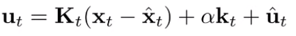
Why does this help? Well, if you look at it recursively, at $x_1$, nothing is different (initial state), so if $\alpha = 0$, then $u_t = \hat{u_t}$. And it propagates down the line. So if $\alpha = 0$, your actions don’t change from your previous iteration. The larger the $\alpha$, the more your actions change. You can search over $\alpha$ to get a good result.